Revision Histories for Versions 5.0.0 - 7.2.0

Shown below are VISRAD revision summaries for:

• Version 7.2.0
• Version 7.1.0
• Version 7.0.1
• Version 7.0.0
• Version 6.6.0
• Version 6.5.0
• Version 6.0.0
• Version 5.5.0
• Version 5.4.0
• Version 5.3.0
• Version 5.2.1
• Version 5.2.0
• Version 5.1.0
• Version 5.0.0
• Versions earlier than 5.0.0

Next

Version 7.2.0

• A new example problem describing how to build a target mounted to a stalk originating from an OMEGA target mount is provided in the documentation. This new example uses several new capabilities recently added to VISRAD. In this example,a hohlraum is set up for the OMEGA target chamber with the following characteristics:
  • The hohlraum is aligned along the P6-P7 axis.
  • The hohlraum cylinder is mounted to a stalk originating from TIM #3.
  • A flat region is cut into the side of the hohlraum.
  • A backlighter is located above the flat region on the side opposite from TIM #5.
  • A hole is cut into the hohlraum to provide a line-of-sight that passes through TIM #5, the flat region, and the center of the backlighter.
  • The hohlraum wall is viewed through one of the LEHs with Dante.
• OMEGA-EP Chamber: Target Mounts TPS7 and TPS83 have been added.
• X-TVS/Y-TVS Viewer: The viewer now automatically detects "Stalk objects" (i.e., Cylindrical or Cone objects used to model stalks that hold targets). This provides a coordinate system for rotating target components using the Target Mounts in the OMEGA and OMEGA-EP target chambers. The criteria for identifying a VISRAD target component as a Stalk for a Target Mount is: 
  • The object must be a Cylinder or a Cone.
  • It must be (nearly) co-aligned with the Target Mount axis.
  • It must use the Target Mount as its Reference Coordinate System.
• NIF Chamber:
  • The blue/green/red cone visibility, power on/off, and power fraction are set using the NIF Beam Parameters dialog (below) are now saved to the workspace file.
  • In the NIF Beam Parameters dialog, when the visibility of a cone is turned on, the power for that cone is automatically turned on. When the power for a cone is turn off, the visibility is automatically turned off.

• Adaptive Mesh Refinement (AMR) modeling: When computing the laser intensity distribution on a target, AMR gridding can now be used. This procedure automatically refines the grid at locations hit by the laser beams. When used, the grid is subdivided using a submesh of triangular elements.
  • To view the laser intensity using AMR mesh, select Display | Direct Laser Power Deposited | AMR Grid.
  • Parameters used in controlling the grid subdivision can be set in the Preferences dialog.
  • The AMR intensities within the subgrid of a surface element are displayed in the VISRAD Main Window. The AMR incident laser intensity results for the sub-grid elements are summed for each surface element and used in:
    • Radiation flux calculations.
    • Results shown in the Surface Elements Table.
  • At AMR subgrid level:
    • Picking to get individual surface element data (using the button) is supported. Except for Incident Laser Intensity, all quantities in the Surface Element Parameters dialog refer to standard grid values.
  • Results at the ARM subgrid level are not saved to a workspace.
• Laser beam power deposition modeling:
  • When integrating the power incident on a surface element, a new integration stencil is now being used. At each point on the surface element where the laser intensity is evaluated, a check is made to see if there is an unobstructed line-of-sight to the beam port. Previously, only the line-of-sight from the surface element centroid had been tested.
  • With the new stencil, results can differ from previous versions of VISRAD. For objects utilizing coarse grids, differences in incident laser powers can differ by several percent. For simulations where objects use a finer grid resolution, differences with previous versions of VISRAD are minimal.
  • An upgrade has been added for situations involving a beam spot that is much smaller than the surface element it is hitting. In this situation, where the beam misses all points on the integration stencil of the surface element, the beam power is now deposited onto that element.
• The capability for specifying the view in the VISRAD Main Window has been updated. Users can now set the Scene location (the point which is being looked at) as well as the Viewing location (the position at which the viewer's eyes are located). This is shown schematically in the illustration below.

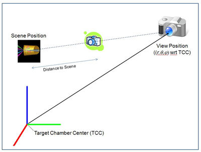
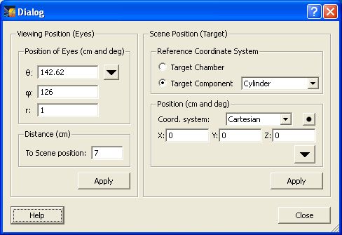
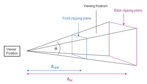
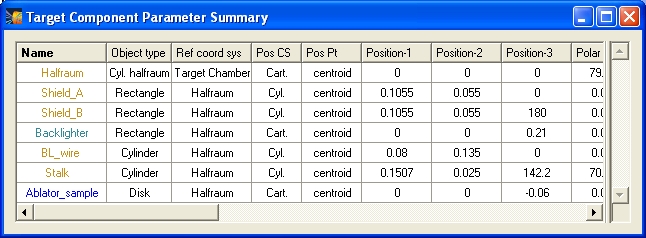
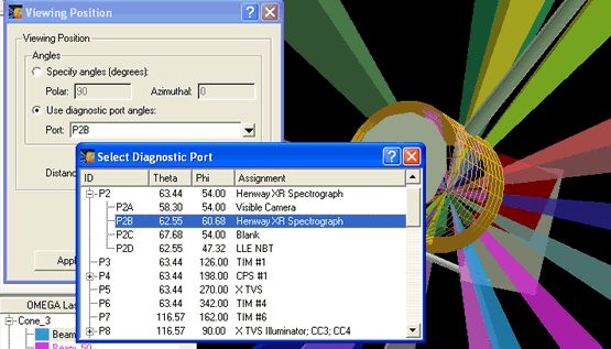
The Viewing position is specified in the Target Chamber coordinate system using spherical coordinates, (r,q,j), as was done previously. The angles can easily be set to those of one of diagnostics ports (using the adjacent button). Also, the zoom factor is automatically adjusted using the user-specified Distance to Scene Position (see illustration above).

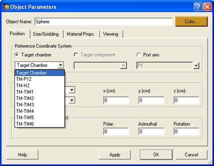
The Scene position can be specified using the Target Chamber coordinate system or the coordinate system of any target component. Given the reference coordinate system, the position can then be can be specified using a Cartesian, cylindrical, or spherical geometry. The user can also easily specify the Scene position to be one of the key points of a target component (using the adjacent button).

• Coordinate System Transformation Tool: A new tool has been added to facilitate coordinate transformations. Users specify a Base (or original) coordinate system, the position of a point in a Base coordinate system, and the New coordinate system. The position of the point in the New coordinate system is then provided when the Update button is pressed.

• Line-Target Intersection Points Tool: A new tool has been added to compute the intersection points of a user-specified line with all target components. The user specifies the Start and End points of the line using one of a variety of coordinate systems. When the Update button is pressed, each intersection point position (in the Target Chamber coordinate system) is shown in a list at the bottom of the widget. An intersection point can also be readily transformed to another coordinate system by invoking the Transport Position button ().

• Individual (Picked) Surface Element Properties dialog: A button () has been added that initializes and displays the Coordinate System Transformation Tool to facilitate getting the surface element centroid position in an arbitrary coordinate system.
• Printing/Exporting images: The color bar can now be included when printing or exporting images of the Main Window graphics. This feature can be enabled or disabled in the Graphics tab of the Preferences dialog (accessed by Edit | Preferences).
• Surface Elements Statistics Dialog: Spherical Harmonics coefficients for the incident flux onto a Sphere object can now be calculated. Coefficients up to l = 4 are displayed. To display the expansion coefficients:
  • Compute the incident flux (select Display | <temperature or flux > menu item)
  • Select the View | Surface Elements Data menu item (in VISRAD Main Window)
  • In the Surface Elements Properties dialog:
    • Set the Target Component to the spherical object name
    • Select the Analysis | Statistics | Incident Flux menu item.
    • Choose the Spherical Harmonics button. (Alternatively, fits to a Legendre series expansion can also be displayed.)

• Laser Beam Parameters Dialog: The buttons in the Apply Values (This Tab Only) To box ("This Beam", "Beams in Cluster", and "All Beams") have been removed to reduces window space required by the dialog. The functionality of these buttons is supported by selecting one or more beams in the Laser Beams List, and in the right-click menu (for example, select Set Pointing).
• Target Component Positions Dialog: Target component positions can now be displayed in Cylindrical geometry, as well as Cartesian and Spherical geometries.
• Available SRF Data Viewer: A calendar pop-up can now be used to edit dates.
• The keyboard shortcut for View | Target Component Positions has be changed to Ctrl+A to avoid conflicts.
• When using the View Location Navigation Control ( in the Main Window), the mouse-controlled rotation and translation values are now reset to zero.
• VisRad was upgraded to utilize advanced version of user interface software library. Required for ongoing and future development.
• Bug fixes:
  • On Mac platforms, the bug occurring when starting VISRAD by double-clicking on a workspace file has been fixed.
  • Crash occurring when selecting Target Component button for the Reference Coordinate System in the Object Parameters dialog has been fixed.
  • NIF Modeling: In the Power Summary dialog, the Power Source for All Laser Beams is now corrected for the fractional power of blue/green/red beam cones that have their power off.
  • The View menu item for the X-TVS/Y-TVS Viewer is now properly enabled for the OMEGA EP target chamber.
  • In the Target Component Positions dialog, when the Target Chamber = "None", the option to display positions using a Diagnostic Ports coordinate system is no longer available (avoids crash).
  • A bug associated with the position of Box clipping volumes has been fixed (bug affected versions 6.6.0 to 7.1.0).
  • The Laser menu is now disabled when Target Chamber = "None" (avoids crash when adding a custom laser beam).
  • Crash occurring when utilizing GENERIZED_MESH objects (from STEP CAD files) and previously saved in VisRad workspaces has been fixed (affects version 7.1.0 only).
  • Problem occurring when deleting a laser beam cluster when only one cluster exists has been fixed.
  • Problem occurring when viewing the Laser Beam Summary table when the Target Chamber = "Custom" has been fixed.
  • Use of mouse-controlled Rotation in Main Window graphics: Upgrades were made to eliminate problem occurring when viewing vector (from Viewing position to Scene position) was co-aligned with the z-axis.
  • In Configure Simulations Parameters dialog, Surfaces tab, problem occurring when adding a surface and then canceling has been fixed.
  • Error occurring when exporting data from the Laser Beam Summary table for non-OMEGA target chambers has been fixed.

Version 7.1.0

• Target Setup: The capability to automatically re-adjust the Position and Orientation Angles of an object when changing its Reference Coordinate System has been added. To do this, check the box at the bottom of the Position tab in the Object Parameters Dialog. The Position and Orientation Angles are then transformed such that the target component does not move. This capability facilitates building a target in one coordinate system, and then re-referencing to a different coordinate system.

• Individual target components can now be shown or hidden in the VISRAD Main Window. In addition, they can also be selectively included or ignored in calculations (i.e., simulation of laser deposition and radiation fluxes). To do this, select the relevant objects in the Target Components List, and right-mouse click. Then select one of the following:
  • Show
  • Hide
  • Include in calculations
  • Ignore in calculations

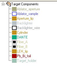
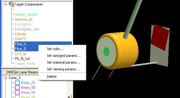
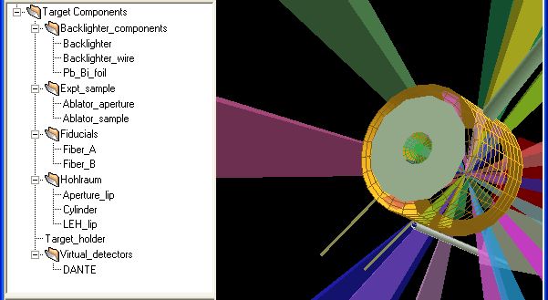
Icons are listed to the left of the objects in the Target Components List (see example above). Their meanings are:

• () Filled and color => Visible and Included in calculations
• () Unfilled and color => Hidden and Included in calculations
• () Filled and no color => Visible and Ignored in calculations
• () Unfilled and no color => Hidden and Ignored in calculations
• STL-formatted CAD files can now be imported and exported by VISRAD.
  • The file extension is ".stl" or ".STL".
  • One or more VISRAD objects can be exported to a single STL file.
  • When importing into VISRAD, the data is represented by a single VISRAD object (a GENERALIZED MESH object), which is given the name filename_nn, where nn is the first unique number for an object of that name.
  • To import from a STL-formatted CAD file, select File | Import CAD File.
  • To export VISRAD target components to a CAD file, select the objects to be exported in the Target Components List. Then, either right-mouse click and select Export to CAD File, or select the Target | Export to CAD File menu item.
• Importing data from STEP-formatted CAD files: Contents are now imported as a single VISRAD object. Attempting to import as multiple VISRAD objects is no longer supported. The new object is placed in the "Target Components" folder of the Target Components List (a new folder is no longer created).
• The wireframe in contour plots is now hidden on initialization.
• The intersection of laser beam cones with a target component can now be displayed on its Surface Elements contour plot. To do this:
  • select View | Surface Element Data in the VISRAD Main Window to show the tabulated results for surface elements;
  • select Plot | <quantity> in the Surface Element Properties dialog to show the contour plot;
  • select View | Beam Spots in the contour plot widget to show the beam spots.

• OMEGA Beamline 25 HR Pickoff: When the 2w/4w beam propagates along BL-25 and is intercepted by an HR pickoff and re-directed to port P9, the beam is represented by a Custom Laser Beam in VISRAD.
  • To be exported properly to an SRF data file, the beam is required to be named "Beam_25_P9".
  • When importing data from the LLE SRF database, whether directly from the database or from an XML-formatted file generated by the SRF-DB, a custom beam is automatically generated with the name "Beam_25_P9", and is placed in a cluster named either "2w Beam" or "4w Beam".
• OMEGA EP Chamber:
  • Diagnostic ports have been updated: based on data in "EP TC Ports 10-1-08.xls".
• ORION Chamber:
  • Diagnostic ports have been updated: based on data in "PORTS28.xls".
  • For Petawatt beams, the portions of cones between the chamber entry points and the off-axis parabolas (OPAs) can now be displayed. To show/hide these cone portions, select menu item Lasers | Pre-Reflection Cones | Show/Hide.
  • For the driver (long-pulse) beams, the beams now originate at a larger distance (2.4 m) from the target chamber center.
• Upgrade to Import of Laser Beam data from OMEGA SRF Database (Focusing and Focusing Units):
  • In cases where Focusing Units are um (spot size), the VISRAD Focus Point Offset is set to:
    • Focus Offset = f# * sqrt[ focus ² - 4d_o ²], where d_o = spot radius for DPP (for no DPP, d_o = 0).
    • Focus Offset = 0, if | focus | ≤ 100 microns in cases with no DPP, and ≤ 2d_o for DPP case.

• Upgrades for GENERALIZED MESH objects:
  • The object position (for GENERALIZED MESH objects only) is defined as the centroid of a bounding box which is determined by the minimum and maximum x, y, and z values for vertices of the object. This position is automatically determined when importing data from the CAD file.
  • GENERALIZED MESH objects can now be clipped.
  • The position is now shown in the Target Component Positions dialog.
  • In the Surface Elements Data dialog, surface element positions are shown in the target chamber coordinate system.
• Displaying properties of individual surface elements (picked with mouse in the Main Window): The total incident laser intensity value is now displayed.

• Multi-Timestep Simulations: The Show button in the Simulation Parameters dialog is no longer supported.
• The Set | Motion Controls menu item has been removed.
• A tool button has been added at the top of the Main Window for toggling the display of clipping volumes. It serves as a shortcut for the Show | Clipping Volumes menu item.
• Use of Box and Rectangle objects as a Reference Coordinate System (for another object) when the Box/Rectangle position is specified by one of the corners: All objects now use their centroid position as the origin of their reference coordinate system. Previously, this was not the case only for Boxes and Rectangles when their position was specified using one of their corners. Upgrades were made to support backward compatibility for old workspace files (objects which use a non-centered Box or Rectangle as a Reference Coordinate System have their positions automatically adjusted on input).
• Upgrades were made to avoid unneeded recomputation of the mesh for unaltered target components.
• Target components: A HELIX object is now available.

• A Help button has been added to the VISRAD Main Window (lower right corner).
• Documentation: A section on Troubleshooting has been added. The contents will be built up over time.
• Bug fixes:
  • In the Object Parameters Dialog, when changing the Reference Coordinate System under the Target Chamber button, the object grid is now recognized as being modified (previously, the coordinate system was not recognized as being modified unless another parameter in the Object Parameters Dialog was also modified).
  • In the Surface Elements Data Dialog, upgrades were made to better support displaying and viewing "inner" and "outer" (or "front" and "back") portions of each object.
  • When changing the color of beams, the colors of the pre-reflection portion of the beams are now also changed (relevant to EP and ORION short-pulse beams).
  • Exporting OMEGA SRF Beam Data to anXML file: When specifying pointing using Distance Toward Port, the distance is now written in units of microns (previously it was cm).
  • Orientation angles for Box Clipping Volumes are now being applied correctly (bug occurred in Ver. 6.6.0 only).
  • When importing an object from the Target Components Library in which the position is defined using a point other than the centroid of the object (e.g., the top of a cylinder), the offset from the centroid is now being applied correctly.
  • When duplicating objects, the object transparency and polygon fill mode are copied to the new object.
  • Bug associated with editing ORION Petawatt beams using the Laser Beam Summary Table has been fixed.

Version 7.0.1

• Bug fix: Pointer to laser beam cluster for new EP Beam in OMEGA chamber is now properly set when reading in old workspace file for OMEGA chamber.

Version 7.0.0

• OMEGA EP Chamber:
  • For Backlighter and Sidelighter beams, portions of cones between chamber entry points and off-axis parabolas (OAPs) can now be displayed (see image below). To show/hide these cone portions, select menu item Lasers | Pre-Reflection Cones | Show/Hide.
  • EP short-pulse beams (Backlighter and Sidelighter) f#'s have been changed from 1.8 to 2.0.
  • Beam rotations have been applied to both short-pulse and long-pulse beams.

• OMEGA Chamber: The short-pulse beam from the OMEGA EP chamber has been added to the OMEGA list of beams.
  • The EP beam is named "Beam_EP". It is square and has an f# = 2.0. The beam rotation is included. The beam enters through Port H9 and reflects off an off-axis parabola near Port H7 (see image below). To show/hide the pre-reflected cone portion, select menu item Lasers | Pre-Reflection Cones | Show/Hide.

• ORION Chamber: Port 46 azimuthal angle changed from 215^o to 225^o.
• Support for editing parameters of multiple target components simultaneously had been added:
  • To edit parameters of multiple objects simultaneously, select the objects to be edited in the Target Components List, right-click with the mouse, and select one of the following:
    • Set Color
    • Set Size/Grid Params
    • Set Material Params
    • Set Viewing Params

    

• Setting Size/Grid parameters is only allowed if all objects selected are of the same object type (e.g., sphere, cylinder).
• When multiple objects are selected, values are initially displayed in edit boxes if values of all objects are the same. Otherwise, the box is empty. Check boxes are "3-state", providing values for "checked", "unchecked", and "no state". For "no state", values pertaining to the check box are not saved for any of the objects being edited.
• X-TVS/Y-TVS Viewer:
  • By default, the X-TVS/Y-TVS views for the OMEGA target chamber are no longer rotated 180^o. The X-TVS/Y-TVS views for OMEGA-EP target chamber continue to be rotated by 180^o.
  • A check box has been added to the X-TVS/Y-TVS Viewer to support rotating X-TVS/Y-TVS views by 180^o.
  • Option has been added to turn lighting Off for grayscale rendering. To adjust color and lighting, use the Set | Color/Lighting menu item in the X-TVS/Y-TVS Viewer.
  • Default settings for viewer are now: Render as Grayscale and Lighting Off.

• Support for automatic zooming to display field of views for OMEGA cameras (Narrow Field, Wide Field, Smart, HS Video, Cryo) and OMEGA-EP cameras (Narrow Field, Wide Field) has been added. To apply automatic zooming, use the buttons to the right of the Zoom slider. The field of views for OMEGA and OMEGA-EP are:

• When showing coordinate system axes (menu item Show | Axes), the length of the axes can now be adjusted. To do this, select Edit | Preferences, and set the axes length in the Graphics tab.
• When importing beam data from an OMEGA SRF data file, beams not turned on are moved to the default cluster ("Cluser_1").
• Bug fixes:

  • Problem of scene in Main Graphics Window flipping up/down viewing far from target has been fixed.
  • Problem associated with deletion of multiple objects which contain clipping volumes has been fixed.
  • Problem associated with setting a new target component's color prior to saving it (i.e., hitting the Apply or OK button in the Object Parameters dialog) has been fixed.
  • Tolerance checks in clipping algorithms have been adjusted, and stopping of application is now avoided.
  • Problem occurring when setting non-zero-thickness Rectangle with N_x = N_y = 2 has been fixed.
  • Tool tips for view manipulation widgets in X-TVS/Y-TVS Viewer have been corrected.

Version 6.6.0

• Main window graphics:
  • Support for plotting quantity values on a logarithmic scale in the main graphics window has been added. To do this, double-click on color bar, and check the Plot Log Values box in the Color Bar Settings dialog.
  • Mouse-driven rotation and translation values are now automatically reset to zero upon when specifying the viewing position (performed with menu item Set | Viewing Position).
  • Mouse-driven rotation and translation values can now be reset to zero by right-clicking on Rotation and Translation buttons on right side of Main Graphics Window.
  • The Main Graphics Window displays the target using "perspective" projection (as opposed to "orthographic" projection). The viewing frustum - i.e., the region that is viewed - depends on the opening angle (q) and by the positions of the front and back clipping planes (see image below). Users can now adjust the front and back clipping plane positions by the use of multipliers on Z_near and Z_far. (The opening angle was adjustable in previous versions.) To do this, select Edit | Preferences, and select the Graphics tab (see image below). Adjusting these often fixes "bleedthrough" problems associated with the OpenGL-driven graphics.

• Support for the OMEGA EP Chamber has been added. The OMEGA EP Chamber utilizes 4 long-pulse beams with f# = 6.5, and 2 short-pulse beams with f# = 1.8. VISRAD currently models the short-pulse beams as originating from their corresponding off-axis parabola.

• Improved support for importing STEP CAD files has been added:
  • CAD structures can now be imported as a single target component or multiple target components. When importing as a single target component, the object types is designated to be GENERALIZED_MESH, and are not editable.

• When importing CAD structures as multiple VISRAD target components, a small reference object is introduced, and all components from the CAD file use this small reference object as their reference coordinate system. All objects can then be moved or rotated by adjusting the position or orientation angles of the small reference object. The name of the small reference object is the STEP file name, preceded by an underscore.
• Algorithms for generating target component grids (nodes and surface elements) has been re-written to support future developments. User interface and functionality should not be affected by these changes.
• Laser beam modeling:
• The beam intensity formula now uses a z-dependent value for the supergaussian index to provide for a continuous transition from a supergaussian profile in the near field to a uniform spatial profile in the far field. (see online documentation for Setting Laser Beam Spatial Profiles). The images below show the change in the beam intensity profile for disks at 0 (left), 2, and 10 cm (right) from target chamber center (TCC), where it is seen that the spatial profile becomes nearly flat-topped at 10 cm from TCC.

• Main Graphics Window: Beam cones are now displayed using multiple elements (polygons) in the direction of the beam axis. This results in "curved" conical surfaces (as can be seen in the OMEGA EP image above) which mimic the iso-intensity surfaces of laser beam cones in near field and far field.
  • The number of polygons used in displaying each beam cone is now editable. To do this, select Edit | Preferences, and select the Lasers tab.



• The parameter "Lens radius / R_o at final optics" in the Spatial Profile tab's Advanced parameters (Laser Beam Parameters dialog) is no longer used and has been removed.
• Object Parameters Dialog:
  • The object type (e.g., cylinder, sphere, ...) is now shown at the top of the widget.
  • For objects of type GENERALIZED_MESH (imported from CAD files), the Size/Gridding tab is disabled, as the size and mesh parameters for objects of this type are not editable.
• X-TVS/Y-TVS Viewer:
  • New menu items have been added for printing the X- and Y-TVS images: see File | Print X-TVS Image and File | Print Y-TVS Image.
  • New menu items have been added for exporting the X- and Y-TVS images: see File | Export X-TVS Image and File | Export Y-TVS Image.
• Port Positions Dialog: Port Assignments are now listed for the diagnostic ports.
• Bug fixes:

  • Problem associated with laser power deposition on 2-D flat objects (Disks, Rectangles, and Spoked Disks) with non-zero thickness has been fixed. Tests for occultation by surface elements on the opposing side of these 2-D flat objects had been ignored.
  • Problem that caused crash when deleting a clipping volume, or an object with a clipping volume, has been fixed.
  • Print routines have been upgraded. Laser beams are now shown on printing for wider variety of PC graphics cards.
  • Problem associated with 2D array out of bounds warning when adding a custom beam has been fixed.
  • Problem in computing occultation of a laser beam accurately for surface elements located far from the focus point of the beam has been fixed. Occultation was previously based on direct line-of-sight test from the surface element centroid to the center of the laser beam port. Test is now performed for line-of-sight from surface element centroid to a point at the laser beam port that is offset from the port center. The offset is a function of the radial offset of the surface element from the center of the beam.
  • Crash that occurred when viewing SRF beam groups table when no beam groups are present has been fixed.
  • Memory leak associated with displaying surface element data 2-D color contour plots multiple times has been fixed.

.

Version 6.5.0

• Improved support for importing STEP CAD files:
  • Upgrades have been made to support import of STEP CAD files containing a much wider variety of objects. The object interpreter in VISRAD attempts to map a STEP object into a VISRAD object (e.g., a disk, cylinder, etc.). If a mapping is not found, VISRAD creates an GENERALIZED MESH object that is composed of a series of nodes and surface elements, but is not characterized by object parameters such as Radius or Length. These objects, named "cad_object_NNNN" when imported (where NNNN is an integer), currently have limitations.
  • Support for grids containing GENERALIZED MESH objects includes:
    • GENERALIZED MESH data can be saved in VISRAD workspaces.
    • Laser power deposition can be computed for targets having GENERALIZED MESH objects.
  • LIMITATIONS and KNOWN ISSUES:
    • GENERALIZED MESH object sizes and grids are not editable. Surface normal directions are not editable.
    • When a GENERALIZED MESH object is in the grid, RADIATION TEMPERATURES AND FLUXES MAY NOT BE CORRECT.
  • Clipping volumes, or an target component containing a clipping volume, cannot be deleted. A crash often occurs.
• Main window graphics -- Mouse interactions have changed:
  • When double-clicking on an object in the main window graphics frame, the Object Parameters Dialog appears for the selected object. Object parameters can then be viewed or edited.
  • New control buttons now appearing on the right side of main graphics frame are used to control response to mouse behavior. Clicking a control changes the mouse mode. Then, moving the mouse while pressed results in the following:
    • Normal mouse pointer
    • Zoom in (upward movement) or out (downward movement)
    • Rotation (rotations can also be controlled using sliders in the lower left corner of the main window)
    • Translation
    • View location control (supports viewing specified object from front, back, etc.)
    • Render surface elements as wire frame
    • Render surface elements using front fill.
    • Render surface elements filling front and back sides
    • Select surface element for writing out frequency- and time-dependent incident radiation
    • Display results for picked surface properties.
• Distributed Phase Plates (DPPs) for OMEGA:
  • The list of available DPPs in VISRAD has been updated to support all DPPs currently in OMEGA's SRF database. DPPs and parameters for supergaussian fits to spatial profiles are as follows:

• In addition, Uniform (no DPP) and Custom Supergaussian spatial profiles are supported in VISRAD.
• The default spot size (radius) for OMEGA beams has been set to 50 microns (Diameter = 100 microns).
• Elliptical beam profile rotation angles can now be specified using a OMEGA Port. Mapping of beam rotation angles are currently supported for the following elliptical DPPs:
  • E-IDI-300 (Pent and Hex ports)
  • E-SG4-865 (Hex ports)
  • E-SG10-300 (Hex ports)

• Importing laser beam parameters from OMEGA SRF data file:
  • Default extension for file name changed from "*.srf" to "*.xml".
  • Support added for case when Focus Units = "um (spot size)" and "R multiples".
  • Beams with Group Name = "Ride Along" are now ignored.
• Importing laser beam parameters directly from the OMEGA RID (SRF) Database (OMEGA OPs only):
  • When saving data to the VISRAD workspace file and data has been imported directly from the OMEGA RID Database, the user has the choice of saving either the "Standard VISRAD" laser beam data or the data imported from the OMEGA RID Database.
  • Warning are now displayed when:
    • Focus Units = "um (spot size)" and a DPP is used (conversion to focus offset not available for such cases).
    • Focus Units = "R multiples" and exactly one spherical object is not in the target grid.
    • The DPP name is not supported by VISRAD.
  • Beams with Group Name = "Ride Along" are now ignored.
• Laser Beam Spot Overlays:
  • The position of labels displayed for laser beam spots can now be adjusted. To do this, adjust the label offset value in the Graphics tab of the Preferences dialog (see below right). To show the Preferences dialog, select Edit | Preferences.

• New features for target component setup include:
  • Curved corners can be specified for Cylinders, Cylindrical Hohlraums, and Cylindrical Halfraums.
• Torus objects are now supported.

     

• Multiple Target Mounts are now supported by VISRAD. Target components can now be set up in the coordinate system of the Target Chamber, or in the coordinate system of a target mount. For the OMEGA laser system, the following Target Mount coordinate systems are now supported:
  • P12
  • H2
  • TIMs 1 through 6

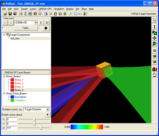
  (One of the primary motivations for supporting this capability is to accurately simulate views for X-TVS and Y-TVS when multiple Target Mounts are used.)

• An example workspace for an OMEGA halfraum utilizing multiple stalks has been added to the VISRAD Examples folder.
• X-TVS/Y-TVS viewer: New capabilities have been added for:
  • Simulating manipulation of targets using multiple Target Mounts.
  • Determining the distance between points picked with the mouse.
  • Automatically adding reticles at beam pointing positions.
  • Printing a composite of X-TVS and Y-TVS views, along with a list of reticle parameters.
  • Multiple selection of reticles in the Reticles list, which supports showing, hiding, or deleting one or more reticles.
  
  The scenes in the X-TVS and Y-TVS windows support target manipulation using multiple Target Mounts. The views support rotation about a stalk axis, and x,y,z-translation using the coordinate system defined by the stalk axis.

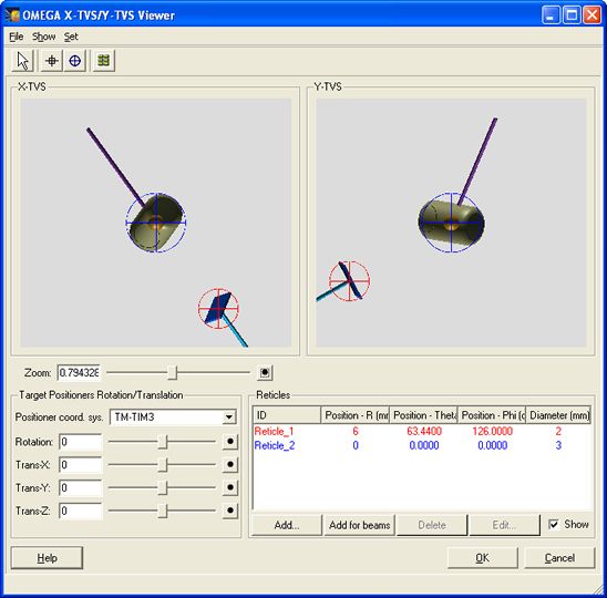
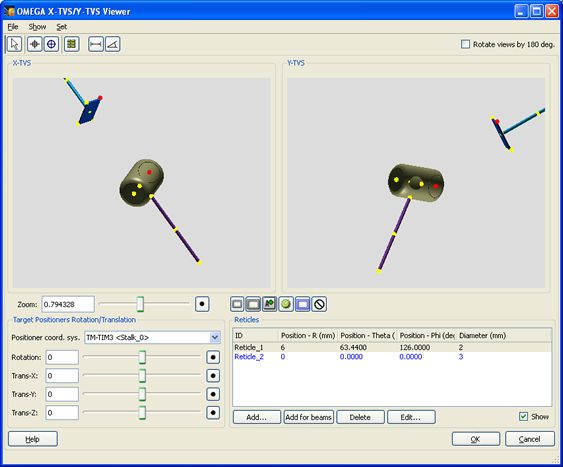
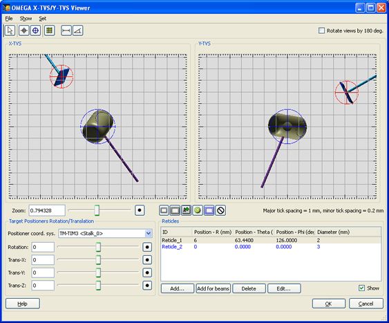
Toolbar buttons in the X-TVS/Y-TVS viewer are used to set the mouse mode for showing target component "key point" positions and displaying distances between then, and controlling reticles. Tool buttons are shown below.

• The left-most arrow is the standard mouse pointer.
• The second button shows the key points (i.e., key locations of target components), and sets the mouse mode for picking key points.
• The third button shows reticles, and sets the mouse mode for controlling reticles (moving, changing size, etc.)
• The right-most button displays the positions of key points for each of the objects.

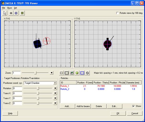
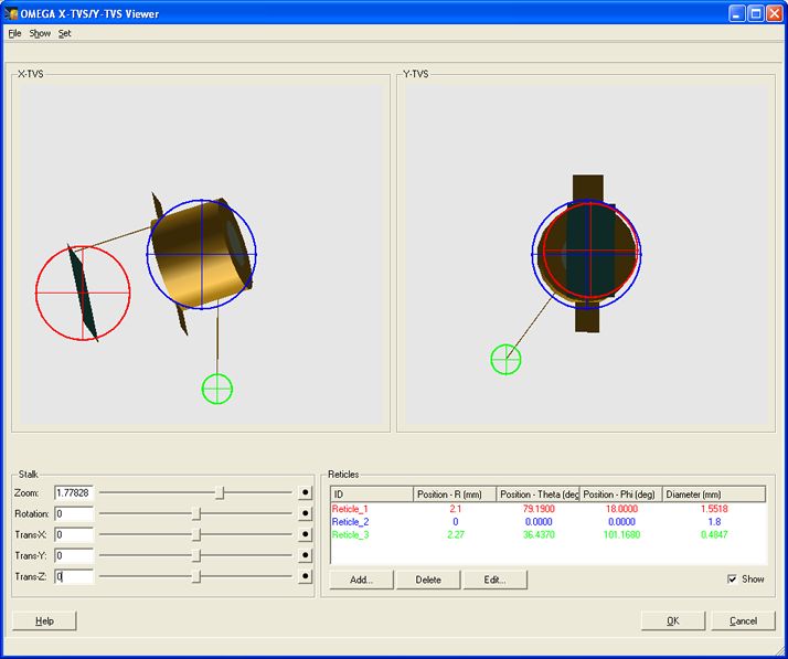
The images below shows an example of reticles positioned at the centroids of two target components. (Note: to view the positions of target components, press the tool button at the X-TVS/Y-TVS Viewer, or select View | Target Component Positions in the VISRAD main window.)

To view the Key Point positions for target components (e.g., top, bottom, and centroid of a cylinder; or corners of a rectangle) select the Key Points tool button (second button from the left).

• To get the distance between any two key points, select them with the mouse, and then with the right mouse button, select Show Distances. (When key points are picked, their color changes from yellow to red.)
• To turn off key points, select the Mouse Pointer button.
• To reset the key points so that none are picked, press the Key Points button.
• The size of the key point rendered in the viewers can be adjusted using the Set | Key Points Size menu item in the X-TVS/Y-TVS viewer.

 

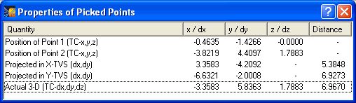
The distances between two Key Points are shown in a widget (see below). The following information is displayed:

• Position of first picked point: r-, q-, and j-position in Target Chamber coordinate system.
• Position of second picked point: r-, q-, and j-position in Target Chamber coordinate system.
• Projected distance (dx, dy, and total distance) between the two points in the X-TVS window .
• Projected distance (dx, dy, and total distance) between the two points in the Y-TVS window .
• The actual distance (dx, dy, dz, and total distance) between the two points in the Target Chamber coordinate system.

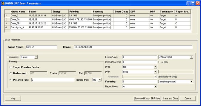
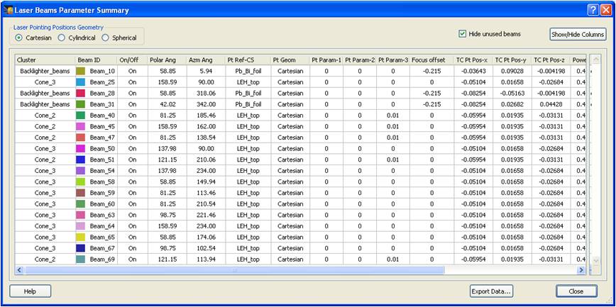
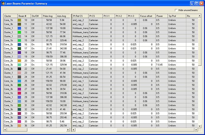
Reticles at the beam pointing positions can be added to the list of reticles in the X-TVS/Y-TVS viewer. To do this, press the Add For Beams button located below the Reticles list. Reticles added have the following properties:

• A reticle is added for each laser beam cluster (or SRF beam group)
• Reticles use name of their associated laser beam cluster
• If beam pointings in a given cluster are inconsistent, a warning is displayed.
• Reticle diameters are 1.0 mm.

• Lasers menu: A menu item has been added to show all beams that have power turned on. To do this, select Lasers | Show All ON Beams.
• Support for multiple selection of target components:
• Deletion of multiple target components is now supported.
• Folders containing target components can now be deleted (previously, folder had to be empty).
• Bug fixes:
  • Problem associated with duplicating target component containing clipping volumes has been fixed (had resulted in bad pointer crash on editing the clipping volume).
  • Problem associated with generating Sphere objects with non-zero thickness has been fixed.
  • Port indices associated with laser beams for the ORION laser beam system has been fixed. Port positions for ports 50-57 and 127, 129 have been updated.
  • Reticle picking updated to more accurately pick with mouse.
  • End-of-file checks have been added in several places to deal with corrupted workspace files.
  • Multiple laser beam editing: Tolerances used when checking for consistency of parameters have been adjusted upward slightly.

Version 6.0.0

• Support for importing STEP CAD files has been added (previously supported in "beta" form only). VISRAD supports importing a limited set of common geometric structures (e.g., sphere, cylinders, etc.), but does not currently support components with arbitrary shapes (e.g., NURB or Bezier surfaces). To import a file, select File | Import Step CAD File.
• The intersection of laser beams with target components can now be displayed. The beam ID is shown in the display (see below examples for a spherical target (left) and hohlraum target (right). To use this feature, select Show | Beam Spots Overlay in the Main Window.

• The points of intersection of the centroid of each laser beam cone with a target can be exported to a file. To do this, select File | Export Beam-Target Intersection Pts.
• Support has been added for exporting VISRAD laser beam data to a file that can be imported into the OMEGA Shot Request Form (SRF) database. Data is written to an ascii file using an XML format. Initially, the only parameters that are actually used in VISRAD that get automatically mapped to the SRF database are pointing parameters (Pointing Position and Focusing) and the Distributed Phase Plate (DPP) ID. Other parameters that are used in the SRF (but not used by VISRAD) can be specified at the time the data is exported (using the widget below). Laser beams in VISRAD Clusters are automatically mapped into SRF Beam Groups. To export VISRAD data for a file that can be imported into the SRF database, select File | Export OMEGA SRF Laser Beam Data.

• VISRAD can now import data from a file created by the OMEGA SRF database. Initially, only laser beam pointing parameters (Pointing Position and Focusing) are utilized. Laser beam pointing parameters currently existing in VISRAD are overwritten when the SRF data is imported. To import an SRF data file, select File | Import OMEGA SRF Laser Beam Data.
• Two options have been added for specifying the pointing of laser beams: pointing to Target Chamber Center, and specifying the Distance Toward a Port. These pointing options are consistent with those used in specifying laser beam pointings in the OMEGA SRF.

• The Laser Beam Summary Table has been updated to show when beams are pointed at Target Chamber Center (TCC) or a distance toward a port ("D toward H6" in figure below). When specifying a distance toward a port, the distance appears in the pointing position column "Pt X-1".
• Table data in Laser Beam Summary Table can now be exported to a file (select Export Data button).

• Reticle diameters are now displayed in the X-TVS/Y-TVS Viewer.
• An option to display rulers at the edges of the X-TVS and Y-TVS viewers has been added. The rulers can be displayed with or without grid lines (see below). To display the rulers, select Show | Rulers or Show | Rulers and Gridlines from the menus of the X-TVS/Y-TVS Viewer. The units for the ruler can be adjusted by selecting Set | Ruler Units.

• Reticle parameters can now be exported to an ascii data file. To do so, select File | Export Reticle Data from the menus of the X-TVS/Y-TVS Viewer.
• Modifications have been made to support faster start-up of VISRAD and lower initial memory needs.
• Laser Beams List in Main Window: Upgrades have been made to better track the open/close status of each cluster when beams are moved between clusters.
• Bug fixes:
  • Diplaying of NIF beams in Main Window now utilizes more polygons to provide for improved display when only a portion of a beam hits a target component.
  • Problem of scene in Main Graphics Window flipping up/down viewing far from target has been fixed.
  • Problem that sometimes occurred when attempting to write too many rows to Surface Elements Table has been fixed.

Version 5.5.0

• OMEGA diagnostic ports have been updated (now based on Jan. 2007 list from OMEGA OPS team).
• File used in providing laser beam data to OMEGA SRF database has been updated to include beam spatial profile parameters.
• X-TVS and Y-TVS views have been rotated 180 degrees to be consistent with OMEGA OPS viewing.
• A table summarizing parameters of all target components has been added. To view the table, select menu item View | Target Components Summary., or use the tool button (). To edit the properties of a target component, either double-click or right-mouse click on the target component in the summary table.

• The background color in the main window can now be specified by the user. To do so, select Set | Background Color. The background color is saved in the workspace file.
• Reticle positions in the X-TVS/Y-TVS viewing dialog are now specified using a spherical coordinate system.
• Mouse-controlled reticle movement in one TVS viewer is now automatically update in other TVS viewer.
• Thickness of reticles in X-TVS/Y-TVS viewers has been decreased.
• Crosshairs have been added to reticles.
• Tool button for X-TVS/Y-TVS viewer is disabled for target chambers other than OMEGA.
• Bug fixes:
  • Problem of writing Cluster Name to workspace file, custom laser beam file, and SRF data file (which occurred only in ver. 5.4.0) is fixed.
  • Laser Beam Summary Table: Selecting Edit Beam with right mouse click is now enabled.

Version 5.4.0

• The X-TVS/Y-TVS Viewer for the OMEGA target chamber has been upgraded. Upgrades include:
  • Both X-TVS and Y-TVS views are shown in the same window.
  • Reticle positions are now defined in the target chamber coordinate system. This establishes positions for both the X-TVS and Y-TVS views.
  • Rotation of target stalk about z-axis is now supported.
  • Translation of stalk in x-, y-, and z-directions (in target chamber coordinate system) is now supported.
  • Zooming of X-TVS and Y-TVS views is now supported.
  • Reticle positions stored in workspaces (prior to Ver. 5.4.0) may not convert to expected positions, as new coordinate system for reticles is now used.
  • Reticles can be re-positioned by dragging with mouse. Positions in both X-TVS and Y-TVS views are automatically updated.
  • Reticles sizes can be modified by selecting reticle with mouse while pressing "r" key, and moving mouse up or down in view.
  • Reticles position in direction perpendicular to view can be adjusted by selecting reticle with mouse while pressing "n" key, and moving mouse up or down in view. Position in other view is automatically updated.

• Laser beam cone transform matrices are now computed for beams that have power OFF, but visibility ON.
• The name on the H6 OMEGA port has been changed from "Y TVS" to "Plasma Calorimeter, Y TVS" to avoid confusion. Y-TVS is at port H6B, one of the H6 sub-ports.
• Bug fixes:
  • Problem fixed that occurred when attempting to view statistics of Surface Elements data (i.e., when selecting the Analysis | Statistics > Incident Flux in the Surface Elements data widget), resulting in 'Array out-of-bounds' message
  • In the X-TVS/Y-TVS viewer, the X-TVS polar angle has been changed from 66.44 degrees to the correct value of 63.44 degrees. (This does not affect the viewing angles or port positions used in the VISRAD Main Window).

Version 5.3.0

• Support has been added to connect to the OMEGA SRF laser beam database at the University of Rochester's Laboratory for Laser Energetics, and use its laser beam parameters within VISRAD. Support includes:
  • Importing and viewing data from the SRF Database.
  • Computing the SRF-DB laser power hitting and missing the target.
  • Exporting laser beam data from VISRAD to a file that can be imported into the SRF-DB (importing tools under development at LLE).
• Users can perform VISRAD simulations using laser beam data contained in the OMEGA SRF Database. This allows users to test whether the laser-target setup using the actual laser beam data entered into the SRF Database. Laser beam data for a particular OMEGA shot is identified by its RID Number.
• The SRF (or SRF-DB) laser beam data is stored in a data structure that is separate from the "Standard" VISRAD laser beam system. This allows users to move back and forth between the Standard laser system and SRF-DB laser system.
• A new menu, OMEGA, has been added to the VISRAD main window. This controls accessing information that is specific to U. Rochester's OMEGA laser system (SRF Database, Phase Plate Library). Some menu items are disabled if the connection test to the SRF Database is unsuccessful.
• A list of OMEGA shot RIDs in the SRF Database can be viewed by selecting the menu item OMEGA | View SRF Shot List.



• Laser beam data from the SRF Database can be displayed and utilized by VISRAD. To view the data, select OMEGA | View SRF Laser Data. The table shows laser pointing and beam spatial profile parameters. When the laser-target interaction is computed, the fractional power hitting and missing the target for each beam is displayed.

• Users can switch back and forth between the Standard and SRF-DB laser systems by selecting either Std. VISRAD or SRF Database from the OMEGA | Set Laser System for Graphics/Simulation menu item.
• Parameters of the Standard VISRAD laser beam system can be exported to a file that is being set up to interface with the OMEGA SRF Database. In the future, it is expected that some portions of the SRFs (Shot Request Forms) will be able to import data from this file. At present, the file contains beam pointing data only.
• Present status of SRF data utilization:
  • Laser beam pointings are fully utilized.
  • Beam spatial profiles for beams using distributed phase plates (DPPs) use nominal spot sizes and supergaussian exponents only. Spatially uniform beams use FOCUS values when FOCUS_UNITS = "um (spot size)".
  • Energetics: VISRAD simulations are based on instantaneous powers, while beam energies are entered into the SRF Database. At present, an estimated power is used based on an assumed 1 ns pulse width.

• For a laser beam with a Uniform spatial profile, the dependence of the radius of the beam on axial distance from the point of best focus, z, has been changed. (Laser beams with non-uniform profiles remain unchanged; see online Laser Beam Profile Properties in online documentation). Previously, for a Uniform beam, the size varied linearly with z:

  d(z) = d_o + ( z / F_L ) ( R_Lens - d_o ) ,

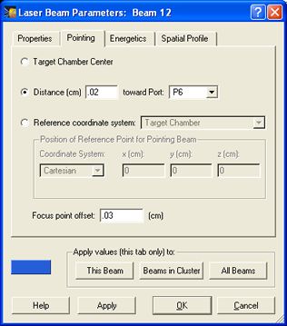
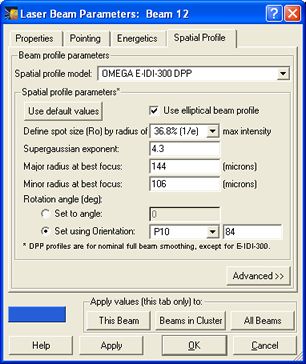
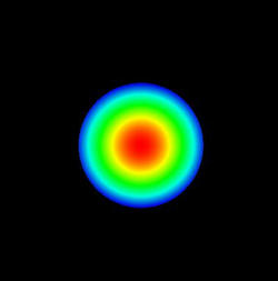
  where d_o is the radius in the plane of best focus, F_L is focal length, and R_Lens is the radius of the final optics. The radius now varies as:

  d(z) = d_o [ ( z / z_o ) ² + 1 ]^1/2,

  where z_o is given by:

  z_o = F_L [ ( R_Lens / d _o ) ² - 1 ] ^-1/2.

  The revised model is similiar to that used for non-uniform beams.

• Bug fixes:
  • Bug fix for crash that sometimes occurs when closing Target Components Library.
  • Color contour plot for Power Source term in Surface Elements Table results widget now plots the correct quantity.

 

Version 5.2.1

• For laser beams with Uniform spatial profiles, dependence of spot size on axial distance from position of best focus, d(z), was adjusted to have same functional dependence as non-uniform beams. See d(z) defined in Setting Laser Beam Spatial Profiles. Previously, the spot size varied linearly with z from the position of best focus back to the final optics.

Version 5.2.0

• A recent paper on Hohlraum Radiation Modeling by D. Cohen et al. is provided in the online documentation (see Appendices).
• A variety of color maps have been added to support the Main Window graphics. To change the color mapping, select Set | Color Bar

  (or double-click on the color bar), and change the Color Map. The images below show the updated Color Bar Settings dialog and an example of simulated laser hot spot emission from an OMEGA halfraum and attached backlighter foil.

       

• The parameters for the SG4 Phase Plate have been updated. The new values are d = 380 microns, n = 3.7, replacing the old values of d = 362 microns, n = 4.2 (see Laser Beam Profile parameters).
• Laser beam profiles now support elliptical beams for OMEGA laser system. Elliptical spatial profiles can be applied to Uniform spatial profiles and Custom spatial profiles. Figures below show beam pattern for test case for disk located at focus (left), 1 mm before focus (center), and 5 mm before focus (right). The eccentricity of the beam is greatest at the focus, and gradually tends towards a circular beam in the near field. (See Laser Beam Profile parameters for additional details.)

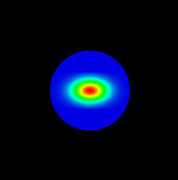
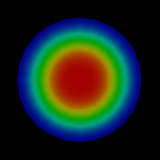
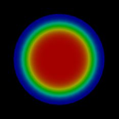
The major and minor axis radii at focus are specified by the user, as is the rotation angle of the minor axis with respect to vertical (see Laser Beam Spatial Profile tab below).

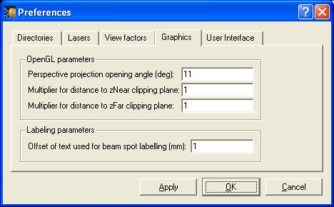
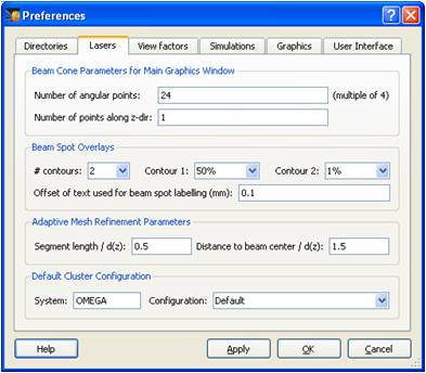
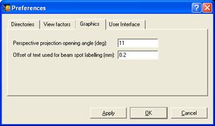
• Preferences: A new tab has been added to set options for the User Interface. Currently, options include: showing/hiding navigation controls for the Main Window, and displaying the Target Components List in color/black text.

  
  
  

• 3-D navigation in Main Window display: Support for mouse- and keyboard-controlled rotating, zooming, and moving display of target has been added. The mouse/keyboard controls are:
  • Return to original settings: Press the 'Esc' key
  • Rotation:
    • about x axis: hold down left mouse button and drag mouse in vertical direction.
    • about y axis: hold down left mouse button and 'Alt' key and drag mouse in horizontal direction.
    • about z axis: hold down left mouse button and drag mouse in horizontal direction.
  • Move: hold down 'm' key and move mouse in desired direction of movement.
  • Zoom: hold down the 'z' key and move the mouse up for increased zoom, down for decreased, or use the vertical wheel on the mouse (if available).

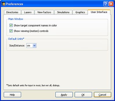
  As users become familiar with the mouse/keyboard navigation controls, they may wish to hide viewing controls previously used for navigation. To show/hide the navigation controls, check/uncheck the appropriate box in the User Interface tab in the Preferences dialog (choose Edit | Preferences).

• The target component list is now displayed in color (default), using the color assigned to the target component. To display the list in black type, see the User Interface tab in the Preferences dialog (choose Edit | Preferences).
• Computational efficiency for displaying color contour plots has been improved.
• NIF beam spatial profiles have been updated to utilize hybrid laser intensity deposition model with rectangular beam profiles
• Bug fixes:
  • Error associated with warning message: "Problem Converting Value to a Double, At Label: Apply multiplier to Column 2 for simulation" in table widget used in setting time-dependent parameters has been fixed.
  • Algorithm for Exporting Images from the Main Window has been updated to work with Lighting disabled.
  • Cone with non-zero thickness fixed for case when inner surface of cone does not require a "disk" at the top.
  • Disk object with non-zero thickness and non-zero inner radius now includes surfaces elements on the inner rim.

Version 5.1.0

• Support for Custom Laser Beams has been added. With this feature, users can add laser beams with arbitrary port locations and f-numbers. Custom Laser Beams have the same properties as fixed laser beams, but have the added feature that the following can be adjusted:

  • Port position
  • Beam name
  • Cone f-number

  Custom beams can be added to an existing laser system (e.g., NIF or OMEGA), or to a laser system containing exclusively Custom Laser Beams.

  Custom Laser Beam parameters are saved in VISRAD workspaces.

  Custom beams can be Imported or Exported to files. This facilitates the re-use of custom beams set up for different VISRAD calculations. To do this, select the File | Import Custom Laser Beams or File | Export Custom Laser Beams menu items.

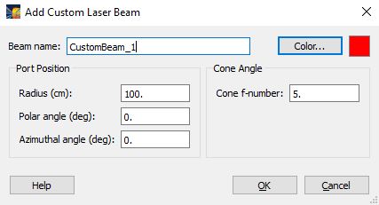
  To add a custom beam, do one of the following:

  • right-click on a cluster in the laser beam list , and select Add Custom Beam
  • right-click on an existing laser beam, and select Duplicate Custom Beam

  When Add Custom Beam is selected, a window is presented in which the beam name, color, port position, and f-number are entered. (Note that these properties can be adjusted later in the Properties tab of the Laser Beam Parameters Dialog.)

  

  .

  Custom Laser Beams are displayed in the laser beams list on the left side of the VISRAD main window. They can be distinguished from fixed laser beams by the diamond symbol located to the left of their name (fixed laser beams have a square symbol). As in the case of fixed beams, the symbol fill/color indicate the beam status:

  • Filled color: beam power is on and shown in display
  • Open color: beam power is on, but hidden in display
  • Open black: beam power is off

  
  
  

  .

• Cutaway views are now supported for the main graphics window. Examples images without (left) and with (right) cutaway clip planes applied is shown below.
  
     

   

• Cutaway views can also be applied when displaying results, such as the radiation temperature or incident flux.

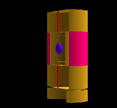
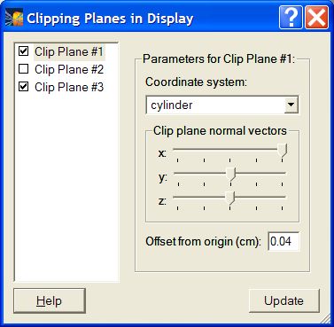
  To set the clip planes used in the cutaway views, select Set | Clipping Planes, or click the Set Clip Planes button on the toolbar. Up to 3 clip planes can be applied. To activate a clip plane, check its box on the left.

  Each clip plane can be applied in the target chamber coordinate system or in the coordinate system of any target component. The clip plane can then be rotated about the x-, y-, and/or z-axis. An offset of the clip plane to the origin of its coordinate system can also be applied.

  
  

• Objects can now be generated that have walls with non-zero thickness. For these objects, the object is constructed with:

  • outer (or top) wall surface elements
  • inner (or bottom) wall surface elements
  • side surface elements

  These objects have surface normals automatically set so that they are directed away from the opposing walls; e.g., the normals of surface elements on the top wall are directed upward, and those for the bottom wall are directed downward.

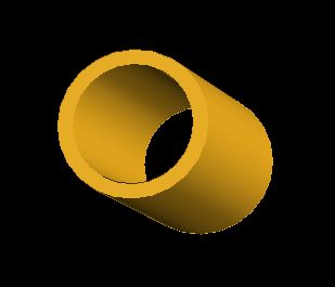
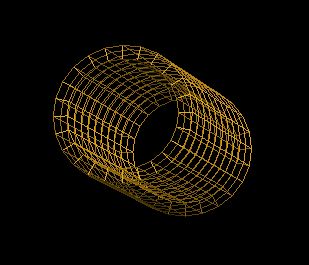
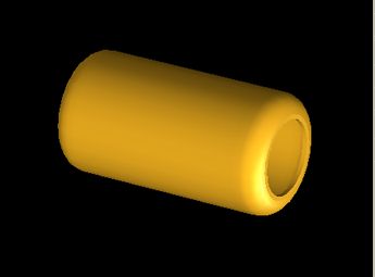
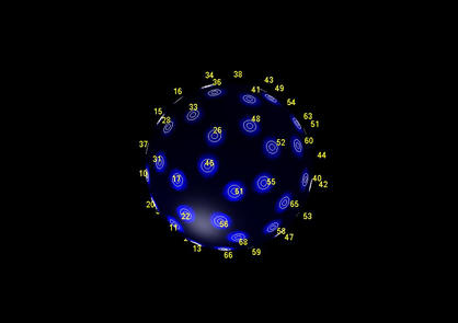
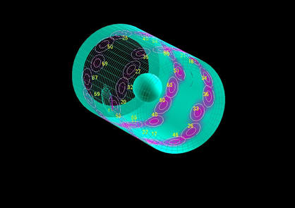
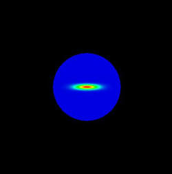
  The images below show a solid (non-zero thickness) cylinder display as wireframe and filled polygons.

      
  

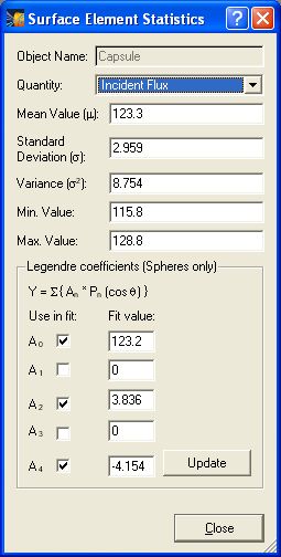
  When displaying results in the Surface Elements Table for objects with non-zero thickness, only the outer (or top) or inner (or bottom) are shown at one time.

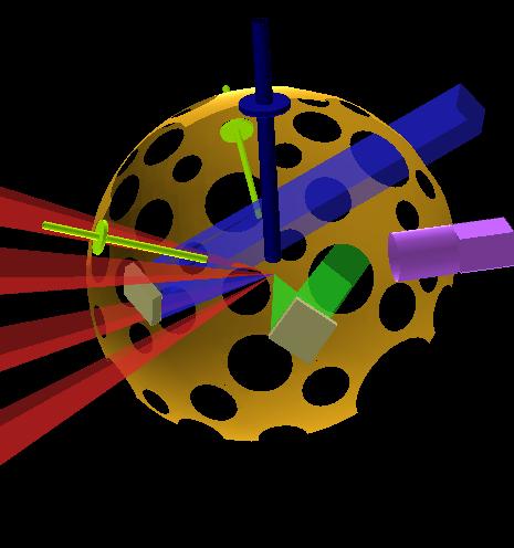
• Support for displaying partially transparent objects has been added for the main graphics window. This is done on an object-by-object basis. In addition, different objects can now be displayed using different polygon fill modes (e.g., wireframe or filled front and back surfaces).

  To set these values, a new Viewing tab has been added to the Object Parameters dialog.

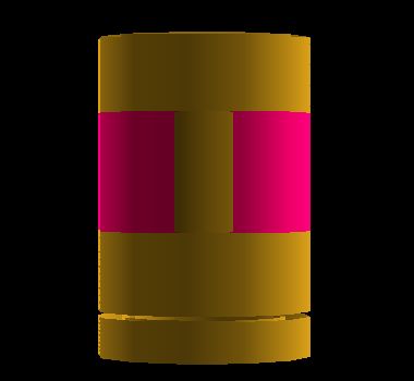
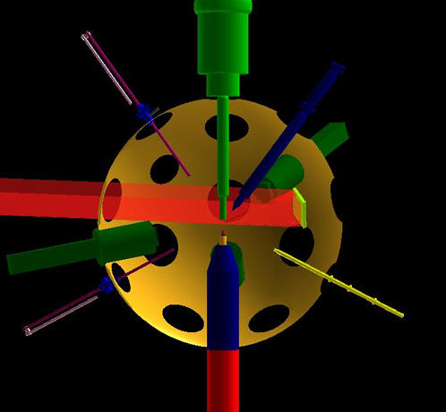
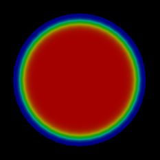
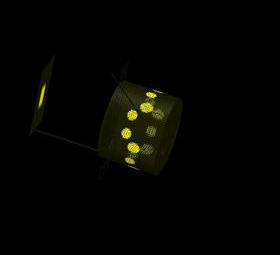
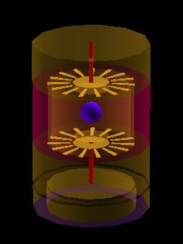
  Example images of partially transparent and non-transparent target systems are shown below.

     

  .

• Additional buttons have been added to the toolbar in the main window to facilitate access to dialogs. From left to right, the toolbar buttons (below) perform the following tasks:
  

  

  • Open a workspace file
  • Save a workspace file
  • Export image from the main graphics frame
  • Show port positions
  • Show laser summary table
  • Show X-TVS/Y-TVS viewer
  • Show surface elements table
  • Add a new target component
  • Delete a target component
  • Clip a target component with a clipping volume
  • Open target components library
  • Show target component positions
  • Toggle coordinate system axes visibility (On/Off)
  • Set viewing position
  • Set the color bar properties
  • Set clipping planes
  • Set polygon mode to wireframe
  • Set polygon mode to front fill
  • Set polygon mode to front and back fill
    
• An option has been added to apply a multiplier for tabulated time-dependent laser powers. This option is displayed when accessing the table from the Energetics tab of the Laser Beam Parameters dialog.
• Fitting of Incident Flux data onto spherical objects has been updated so that users can fit to Legendre polynomial expansions ranging up to P₄.
  • Coefficients used in fitting the flux data are selected by checking appropriate boxes (see bottom portion of widget below).
  • If new coefficients are selected/deselected, press the Update button to display updated fits to the Legendre polynomial expansion.
  
  
  

  .

• Portions of Spheres can now be generated in which limits to the azimuthal angle are specified.
• The simulation time is now displayed at the top of the Surface Elements Table.
• Clipping algorithms updated to better handle situation when clipping volume boundary exactly coincides with boundary of target component.
• Bug fixes:

  • Error in computing variance and standard deviation that is displayed in Surface Element Statistics dialog fixed. Previously displayed values (ver. 5.0.0 and earlier) were too low by a factor of 2 for variance, and by sqrt(2) for standard deviation.
  • Polar angles for Beams 10, 13, 20, 28, 33, 48, 52, 58, 65 and 66 were changed from 58.582 to their correct value of 58.852.
  • Problem of saving renamed folders holding target components has been fixed.
  • Problem associated with poor aspect ratio in main graphics window after opening new workspace has been fixed.
  • Error in algorithm for generating grid for Boxes, when number of grid points in x-, y-, and z-directions is different, has been fixed.
    

Version 5.0.0

• A new widget containing a summary of parameters for all laser beams has been added. To view this, select View | Laser Beams Summary. Features of the table include:
  • Displays parameters for beam pointing, power, and spatial profiles for each laser beam.
  • Beams can be sorted by clicking header of any column.
  • Parameters for one or more beams can be edited by selecting with mouse. Use double-click to edit a single beam. To set parameters for multiple beams, first select beams and then click with right mouse to obtain pop-up menu.
  • Unused beams can be shown or hidden.
  • A splitter is provided to facilitate simultaneous viewing of widely separated columns.

• Target components listed on the left side of the main window can be grouped into folders to facilitate setup for complex target systems. To add a folder, right-click on an existing folder (e.g., Target Components), and select Add folder. Target components can be moved between folders by moving them with the mouse (drag-n-drop).

• The list of OMEGA diagnostic ports has been updated. The updated list now includes sub-ports for pent and hex port locations. The port and sub-port locations can be used when: setting the view position for the main window display; setting reference coordinate system for positioning and orienting a target component; and setting a reference coordinate system for viewing target component positions.

• Capability to set parameters for all laser beams within a single cluster has been added. To do this, right-click on the cluster name, and select popup menu item.

• The "key points" on each target component can now be displayed in spherical coordinates (r,q,j), in addition to previously-supported Cartesian (x,y,z) coordinates. The positions can be displayed in the Target Chamber coordinate system, a coordinate system aligned with any of the diagnostic ports, or the coordinate system of any target component. To access this, select View | Target Component Positions.

• Bug fixes:

  • Laser beams within each cluster are now listed in alphabetical order.
  • In Port Positions widget, sorting has been fixed.