
| CONTENTS | GLOSSARY | SUBJECT INDEX | SEARCH DOCUMENTATION |
User-specific preferences can be specified by selecting Edit | Preferences. Parameters set in Preferences widget are saved in a preferences file, which SPECT3D loads at startup.
Preferences can be used to:
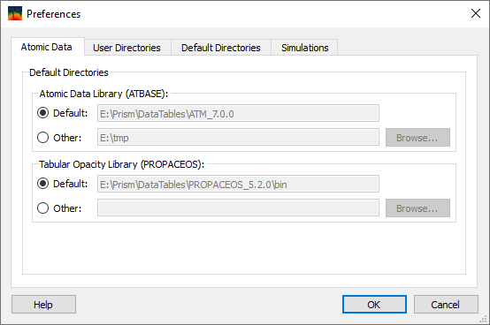
When selecting the Default button for the Atomic Data Library or the Tabular Opacity Library, SPECT3D utilizes the default directory (which can be altered in the Default Directories tab, described below). With the Other button, the user can explicitly set the directory path for each of these libraries.
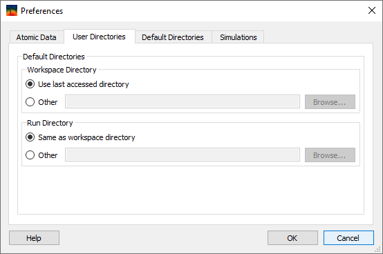
The default directory used for opening workspaces can be either the last directory used by SPECT3D or a user-specified directory.
The default directory used to write simulation output can be either the same as the directory where the workspace is located or a user-specified directory.
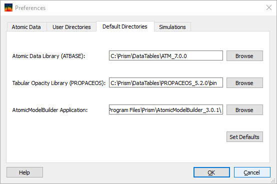
When SPECT3D is run for the first time (in which case no preferences file is detected), default directories for the Atomic Data Library, the Tabular Opacity Library, and the path to the AtomicModelBuilder application are initialized by the SPECT3D application. For Linux and Mac OSX platforms, these paths are set assuming the default Prism applications directory structure. For Windows platforms, they are initially set using the environment variables PCS_ATBASEDATA_DIR, PCS_PROPACDATA_DIR, and PCS_AMB_DIR, respectively, if they exist (they are typically set up during the installation of ATBASE and PROPACEOS data, however environment variables for Windows platforms are editable using System in the Control Panel folder). On all platforms, these default directories are editable in the Default Directories tab, and may need to be changed when:
On systems with more than one processor, the calculation of the opacities for DCA materials can be run in parallel using multiple processors. The option is enabled by checking the Perform multi-threaded simulations box. To limit the number of processors used, check the Limit max number of threads to: check box and enter the number to be used. If this box is not checked or if the number entered exceeds the number of processors available, all the available processors will be used.
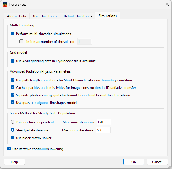
Use AMR gridding data in Hydrocode file if available: this controls the ability to utilize AMR (Adaptive Mesh Refinement) grids generated by Prism's GridConvert application.
Utilizing this type of grid, the CPU required to compute the intersections of lines of sight (LOS) with the plasma grid are reduced significantly (~ 2 orders of magnitude in 2-D r-z test calculations).
Use path length corrections for Short Characteristics ray boundary conditions: a scaling correction is applied for Shortc Characteristics which can significnatly improve accuracy, especially for the optically thin regime. See details in the Appendix Short C Boundary Condition Scaling.
Cache opacities and emissivities for image construction in 1D radiative transfer: for 1D geometries, during the image calculation, opacities and emissivities are cached for each zone, rather than being re-computed for every detector line of sight. This can significantly increase calculation speed.
Separate photon energy grids for bound-bound and bound-free transitions: for atomic rate calculations, using separate photon energy grids for bound-bound (bb) vs. bound-free (bf) transitions can significantly improve calculation speed, e.g. if there are many more bb transitions than bf transitions.
Use quasi-contiguous lineshapes model: uses Stark broadening models were implemented based on the semi-empirical approach detailed in Gu and Beirsdorfer (Phys. Rev. A, 101, 032501). Un-checking will revert to the old Stark broadening model. For more information on the models please refer to a appendix in the documentation titled "Stark Broadening Models in Prism Codes".
Solver Method for Steady-State Populations: if "Pseudo-time-dependent" is selected, the steady state solution of statistical equilibrium is obtained by a time-dependent solver to let the system of ordinary differential equations evolve until equilibrium is reached. If "Steady-state iterative" is selected, a true steady state solution is obtained in each iteration for a given set of collisional and radiative rates. The "Steady-state iterative" solver is more efficient for a broad range of problems because it often requires fewer iterations to converge, and needs less time per iteration.
Use block matrix solver: applies only if "Steady-state iterative" is selected for the populations solver. This is a custom designed linear equations solver grouping a larger number of atomic levels in a smaller number of blocks. Each block typically consists of one ionization stage. The solution to the original system of linear equations is obtained iteratively by solving the populations of blocks. Once the block populations are known, the smaller system of equations for individual levels in each block are solved one block at a time. The iteration continues until the solution of all levels and blocks reaches self-consistency.
Use iterative continuum lowering: continuum lowering and level population are inter-dependent. Versions prior to Spect3D 20.5.0 compute the continuum lowering parameters, such as occupation probabilities and ionization potential depression, using the LTE population assuming no continuum lowering. The Iterative procedure makes the continuum lowering and level populations self consistent.
| Copyright © 2024 Prism Computational Sciences, Inc. | SPECT3D 20.5.0 |