| CONTENTS | GLOSSARY | SUBJECT INDEX | SEARCH DOCUMENTATION |
SPECT3D revision summaries are shown below for:
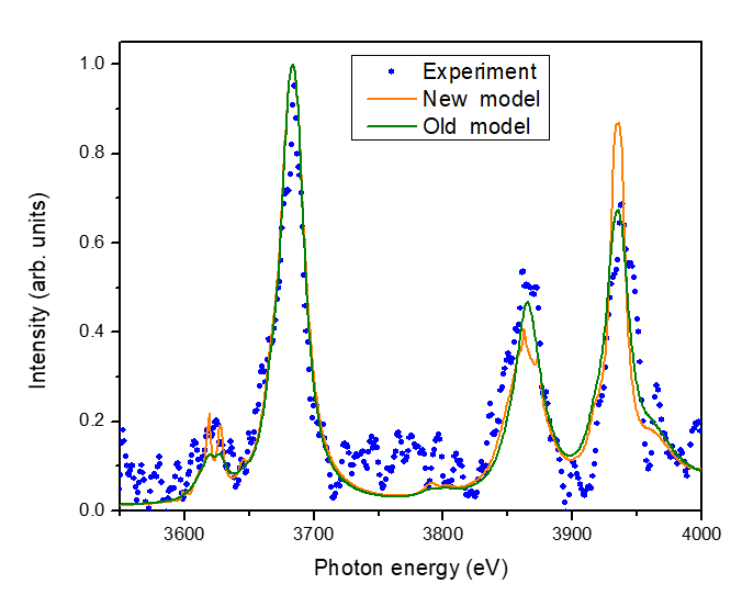
Depending upon plasma conditions and composition, the new Stark broadening model may have a significant impact on the spectral distribution Figures below show the results of the simulations for:
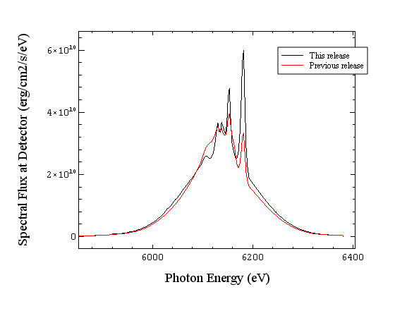
Typical Ar K-shell emission spectrum from ICF implosions
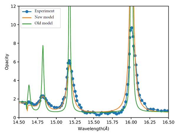
Calculations of Oxygen opacities
In some cases, this change will result in different XRTS spectra, however the new version will be more physical. The following example shows a difference in the XRTS spectrum for a CH plasma at 100 eV and 0.25 g/cc, where C is the 2nd element in the Atomic Data list. Thus, for the previous release, C would be treated as having an average ionization of 5.0, while in this release, it gets that value from Spect3D. Furthermore, this example does not have the "Override mean charge (Z-free)" box checked, and its field value has nothing in it. Thus, for the previous release, H would be treated as having an average ionization on 0.0, while in this release, it gets that value from Spect3D:
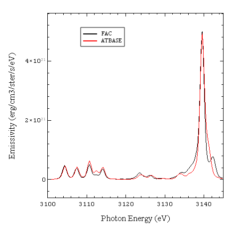
Simulation results for Ar-doped DD plasma at 600 eV temperature and 1 g/cc density computed with FAC and ATBASE data. Ar He-alpha transition and associated Li-like satellites.
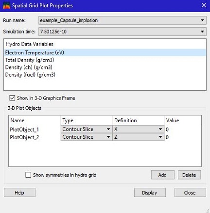
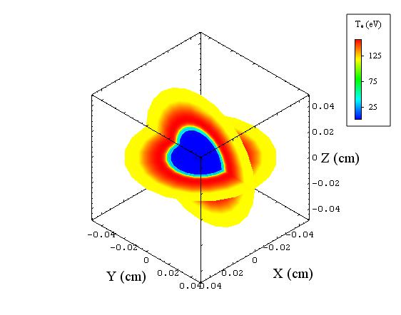
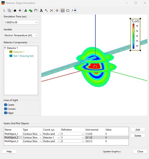
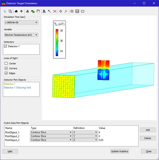
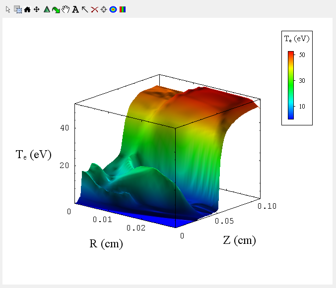
When displaying in 3-D, one or more contour slices and/or isosurfaces can be added to the plot window. The above example shows contour slices of the electron temperature in the x = 0 and z = 0 planes.
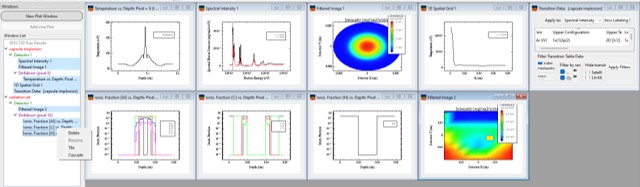
Ionization plot windows are used to show various quantities associated with ionization results from a SPECT3D calculation, including mean charge, ionization fractions, and atomic level populations. The temperature, electron density and material mass densities can also be displayed. The simulation times available are those used in the SPECT3D calculation (in SPECT3D calculations with time-dependent kinetics, the simulation time grid is generally different than the time grid of the hydro data file).
Like the displays of hydro data (above), results can be displayed using either the geometry of the original hydro grid, or using a 3-D spatial grid.
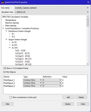
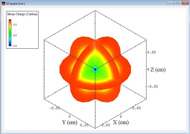
The example above shows the spatial distribution of the carbon mean charge state in the x = 0, y = 0, and z = 0 planes.
When viewing atomic level population results, the Atomic Rate Coefficient data for a particular volume element can be displayed by picking the element after clicking on the (![]() ) button in the toolbar.
) button in the toolbar.
| Copyright © 2024 Prism Computational Sciences, Inc. | SPECT3D 20.5.0 |