Sample Problem: Generation of CH Data

This shows an example of how to compute EOS and opacity data for CH.

The gridding is summarized as follows:

• Temperature:
  • low temperatures: 0.1, 0.3, 0.5, 0.8, 1.0 eV
  • evenly-spaced linearly from 2 to 60 eV at 2 eV intervals
  • evenly-spaced linearly from 60 to 100 eV at 10 eV intervals
• Ion density:
  • 41 evenly-space logarithmically from 10¹⁹ to 10²³ ions/cm³
• Photon energies:
  • 500 groups from 0.1 eV to 10 keV, with group boundaries evenly-space logarithmically.

After starting up PROPACEOS, select the Add button on the upper-right side of the Plasma Elements widget. When the periodic table pops up, select "C". Then, select the Add button again, and select "H" from the periodic table. The Plasma Elements widget should now look like the example below.

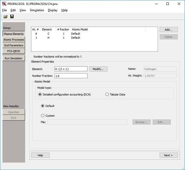
The number fractions for both H and C are 1.0. They can be left this way because the element number fractions entered are normalized to unity at the beginning of the PROPACEOS calculation.

The Atomic Processes widget is left unchanged. The default is a LTE calculation.

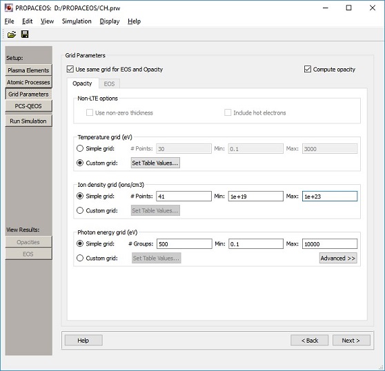
To set up the grids, either select Next from the Atomic Processes widget, or select the Grid Parameters button on the left side of the Main Window.

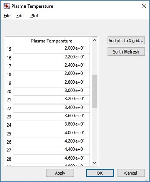
To enter the custom temperature grid, select the Custom Grid radio button. Then select the Set Table Values button and an empty table will appear.

To enter the low temperature grid points, enter values directly into the table.

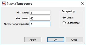
To enter the evenly-spaced points between 2 and 60 eV, select the Add Pts to X Grid button. Then in the popup dialog, select Linear in the Set Spacing area; set 2 for the Min. Value, 60 for the Max. Value, and 30 for the Number of Grid Points. Then press Apply. This will add 30 points to the table, starting at 2 eV and ending at 60 eV.

To enter the evenly-spaced points between 70 and 100 eV, follow a similar procedure, adding 4 evenly-spaced points between 70 and 100 eV.

For the ion density grid, make sure the Simple Grid radio button is pressed. Enter 41 for the number of points, and 1.0e19 and 1.0e23 for the Min and Max values, respectively.

For the photon energy grid, make sure the Simple Grid radio button is pressed. Enter 500 for the number of groups, and 0.1 and 10000 for the Min and Max values, respectively.

It is generally a good idea to save the workspace periodically. To do this, select the File | Save menu item.

To start the simulation, select the Run Simulation button. After entering the run name and run directory, the calculation will start.

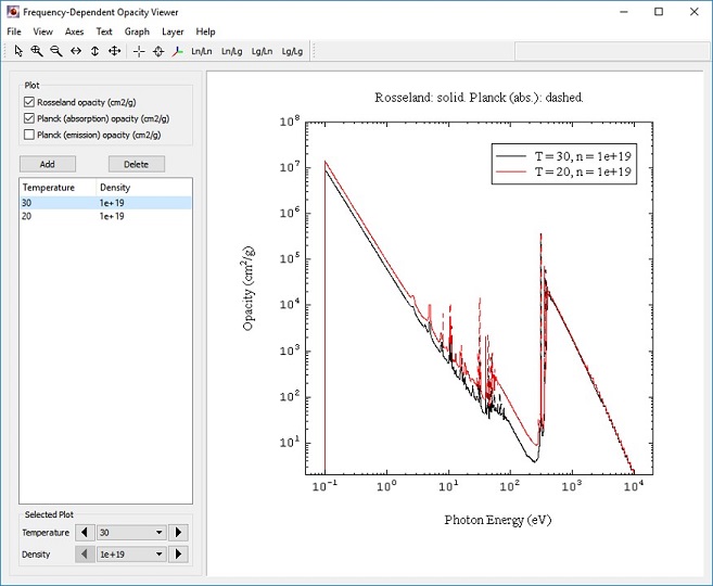
To view results for opacities, select the Opacities button on the left side of the Main Window.

The opacity plots for the first T-ρ point are automatically added to the graph. The temperature or density of the curves shown can be adjusted by selecting the T-ρ point in the list box in the left, and then adjusting the values using either the drop-down combo box or arrows in the lower-left corner of the Opacity Viewer dialog.

To add a second set of curves (a "set" corresponds to all 3 types of multigroup opacities: Rosseland, Planck absorption, and Planck emission), select the Add button, and select from the menu the T-ρ point you wish to add. Doing this allows for comparisons to be made for differing T-ρ conditions.