
| CONTENTS | GLOSSARY | SUBJECT INDEX | SEARCH DOCUMENTATION |
SpectraPLOT can display a variety of SPECT3D results. Plot window types include:
A description of each of these is given below.
For each plot widget type, the units can be adjusted in the Window Quantities/Units Panel.
SPECT3D calculated the specific intensity, Iν, in units of erg/cmˆ2/srad/s/eV, as seen by each line of sight (LOS) defined by the SPECT3D detector pixel centroids.
To produce a frequency-dependent flux, Fν, SPECT3D integrates each LOS's Iν over the plasma solid angle subtended by that LOS's pixel (which amounts to a multiplication by that solid angle), resulting in a spectral flux for that LOS in units of erg/cmˆ2/s/eV. These fluxes are summed over all LOSs (pixels) in the SPECT3D detector plane, resulting in a total flux at the detector position, whose unit is still erg/cmˆ2/s/eV. The data for each spectrum originate from SPECT3D-generated *.sis files.
For more detail on how specific intensity and flux are calculated, see SPECT3D Detector Fluxes.
For more detail on how to relate the flux to a total power collected, see Interpreting Results.
Example spectra are shown below:
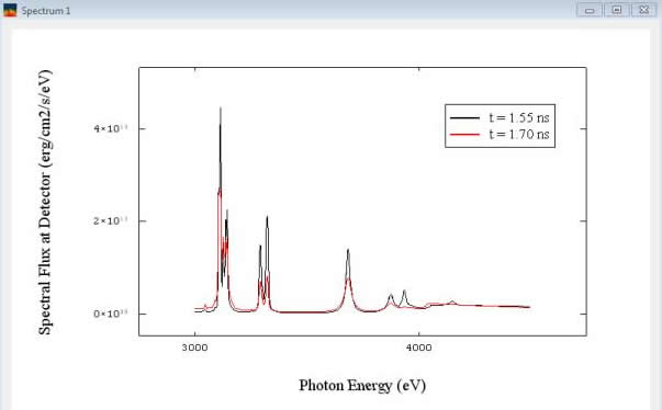
The name of each plot item is used to set the default name in the legend.
Either time-resolved (i.e., Instantaneous) or time-integrated spectra can be displayed. However, note that each of the plot items must all have their Time Settings be either Instantaneous or Time-Integrated. Because of this, if a Spectrum plot widget contains more than one plot item, changing between Instantaneous and Time-Integrated is not allowed.
Editing the parameters for each of the line plot items is done using the Plot Settings Panel. For this plot widget type, the Spectral Resolution for multiple line plots can be changed by selecting items in the Plot Items List, and selecting the right-click menu item Set Spectral Resolution.
A table of atomic transitions used in a SPECT3D run can also be displayed to facilitate determining which transitions contribute to the line emission or absorption in a spectrum.
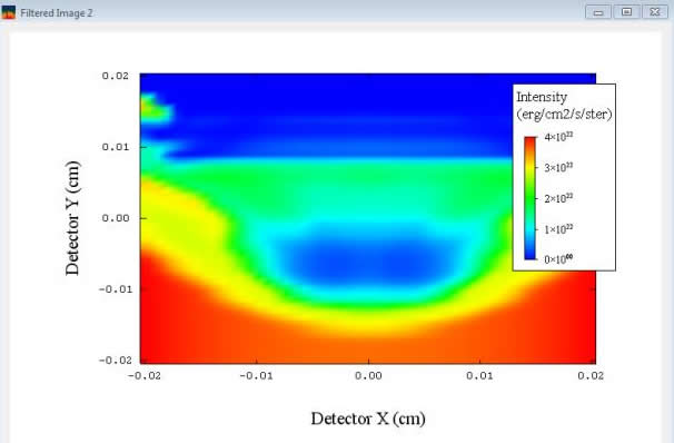
To produce a frequency-integrated intensity image, SPECT3D integrates each LOS's Iν over the frequency range defined by the user in Spectral Grid section. An Image plot displays this value for each SPECT3D detector pixel (LOS), and is thus a map of the intensity (in units of erg/cmˆ2/srad/s) over the solid angle of the plasma. The data originate from the SPECT3D-generated *.dti files and *.bsc files. The *.dti files contain frequency-integrated results, while the *.bsc files contain frequency-dependent results (which are generated for a user-specified number of frequency "bins", the number of which is typically small compared to the number of high-resolution frequency points in a SPECT3D simulation).
For more detail on how specific intensity and flux are calculated, see SPECT3D Detector Fluxes.
For more detail on how to relate the flux to a total power collected, see Interpreting Results.
A *.dti file contains the unfiltered, frequency-integrated (over the user-specified range of the SPECT3D spectral grid) specific intensity computed for each detector pixel. In addition, the *.dti file may contain additional data that can be displayed in Image plot windows. The type of data to be displayed in the plot window is set in the Pixel Data Type box of the Plot Setting Panel.
Because data in the *.dti file is frequency-integrated, frequency-dependent Filtering cannot be applied in Images using the *.dti data.
For SPECT3D runs that utilize a disk detector with circular symmetry, the intensity can be displayed in a Radial Image plot (i.e., intensity vs. radius in a line plot). This option is made available to the user if the the run currently selected in the SPECT3D Run Results List when the Image plot button is clicked utilized a disk detector.
Time-Dependent Flux Plot Window
A Time-Dependent Flux (a.k.a. Light Curve) plot widget holds one or more line-plots of absolute intensities as a function of time. The data originate from SPECT3D-generated *.sis files. The intensities shown are frequency-integrated and summed over all pixels in the 2-D detector plane. Since each point is a frequency-integral of a spectral flux (which are plotted in Spectrum windows), the units are erg/cmˆ2/s.
An example is shown below.
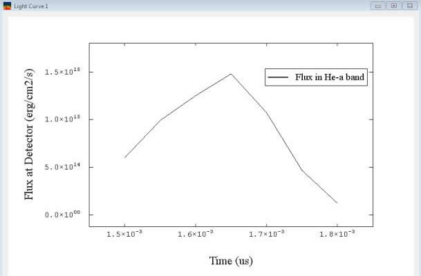
The name of each plot item is used to set the default name in the legend.
Filtering can be applied to show the time evolution of intensities in a particular wavelength band.
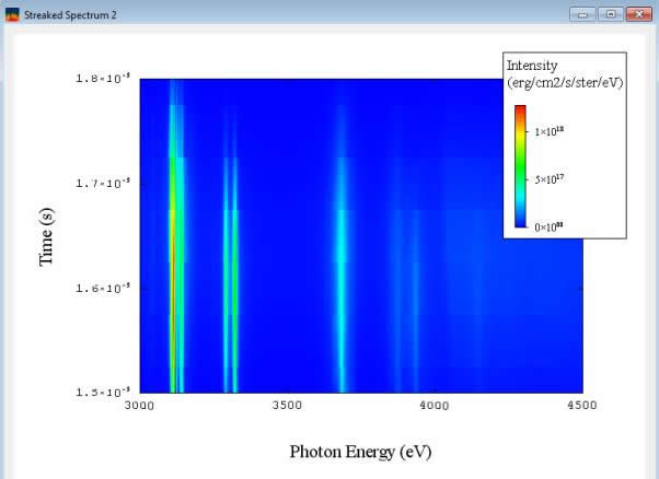
A Streaked Spectrum plot widget contains a contour plot showing spectral flux as a function of photon energy (horizontal axis) and time (vertical axis). It is a way of visualizing the spectral flux at all time steps on a single plot. The units are the same as for individual spectra, erg/cmˆ2/s/eV. The data originate from SPECT3D-generated *.sis files. The intensities are integrated over the 2-D detector plane.
An example is shown below.
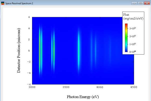
Space-Resolved Spectrum Plot Window
A Space-Resolved Spectrum plot widget contains a contour plot showing spectral flux (as a function of photon energy on the x-axis) at each SPECT3D pixel location in either the horizontal or vertical detector dimension (on the y-axis). The unit is erg/cmˆ2/s/eV (the same as that for a spectrum, which is the summed flux over all pixels). The output for this data must be requested in the SPECT3D interface prior to running the simulation, in the "Spectra" tab of the Output section. Depending on settings used in the SPECT3D simulation, several types of data can be available:
Support for displaying pixel-dependent spectra is also available. When adding a plot widget for Space-Resolved Spectrum, an option to generate a contour plot or line plots (one for each selected pixel) is presented. For line plots, a list of pixel positions is provided. For each pixel selected, a line plot for the corresponding spectrum is displayed.
The data originate from SPECT3D-generated *.srh and *.srv files in the cases of space-resolved spectra in the horizontal and vertical dimensions, respectively, and *.csd files for crystal slit imaging spectra. The intensities are summed over pixels in the second dimension of the 2-D detector plane.
An example contour plot is shown below.
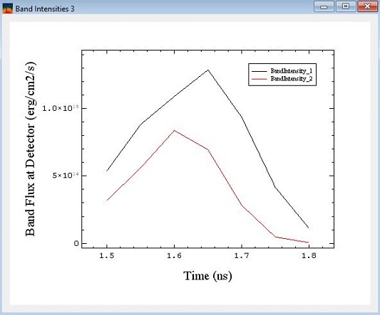
Band Intensity plot windows support displaying Spectral Band Intensities and Band Intensity Ratios as a function of time. In SPECT3D simulations which utilize space-resolved spectra, they can also be displayed as a function of detector pixel position. See Displaying Spectral Band Intensities for more information on setting up spectral bands.
Optical Depth Isosurface Plot Window
An Optical Depth Isosurface plot widget displays one or more isosurface plots. Isosurface plots show the location in 3-D space where the optical depth, for a given photon energy and measured from the detector, reaches the specified isosurface value. The output for this data must be requested in the SPECT3D interface prior to running the simulation, in the Output setup widget. For every combination of (a) photon energies entered into the "Photon Energies" tab, and (b) optical depths entered into the "Optical depths" tab, this data will be written into SPECT3D-generated *.ods files.
An example is shown below for Ar He-β isosurfaces of τ = 0.1 and τ = 1.0 in a capsule implosion simulation, where the detector is located along the +x axis.

Hydrodynmics data (i.e., data that is input into a SPECT3D calculation) can be displayed using either the geometry of the original hydro grid (e.g., 1-D spherical, 2-D cylindrical R-Z, ...), or using a 3-D spatial grid. The simulation times available are those contained in the hydro data file. To plot in 3-D, check the Show in 3-D Graphics Frame check box (see below)..
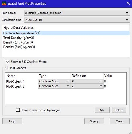
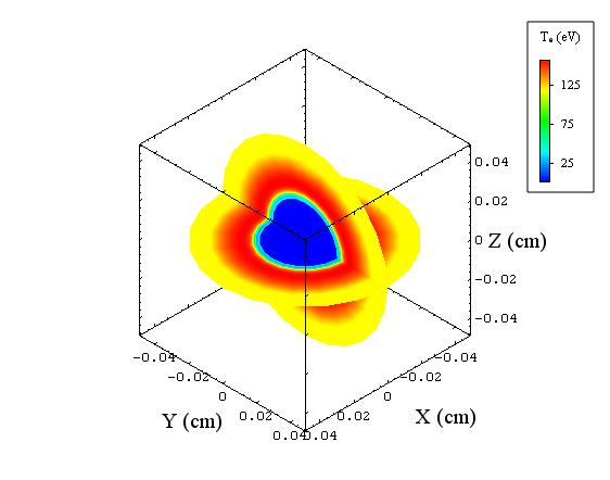
When displaying in 3-D, one or more contour slices and/or isosurfaces can be added to the plot window. The above example shows contour slices of the electron temperature in the x = 0 and z = 0 planes.
Ionization plot windows are used to show various quantities associated with ionization results from a SPECT3D calculation, including mean charge, ionization fractions, and atomic level populations. The temperature, electron density and material mass densities can also be displayed. The simulation times available are those used in the SPECT3D calculation (in SPECT3D calculations with time-dependent kinetics, the simulation time grid is generally different than the time grid of the hydro data file).
Like the displays of hydro data (above), results can be displayed using either the geometry of the original hydro grid, or using a 3-D spatial grid.
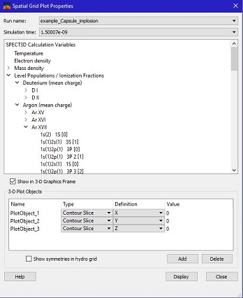
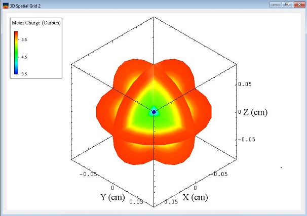
The example above shows the spatial distribution of the carbon mean charge state in the x = 0, y = 0, and z = 0 planes.
When viewing atomic level population results, the atomic rate coefficients for a particular volume element can be displayed by picking the element after clicking on the (![]() ) button in the toolbar. For more information, see Viewing Rate Coefficient Data.
) button in the toolbar. For more information, see Viewing Rate Coefficient Data.
| Copyright © 2024 Prism Computational Sciences, Inc. | SPECT3D 20.5.0 |