Example: Radiation Burn Through SiO2 Foam

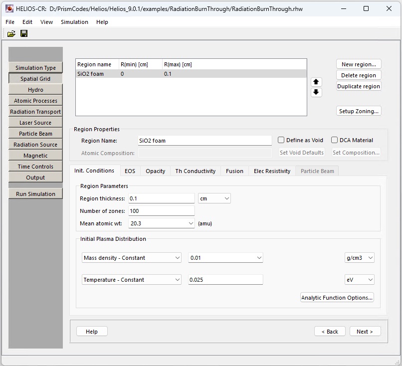
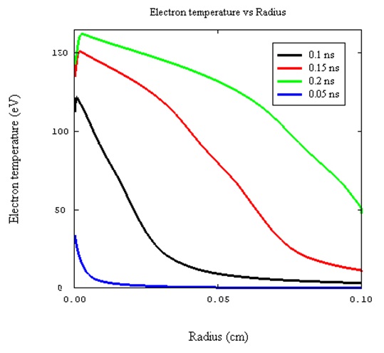
In this calculation, an external radiation source burns through a SiO₂ foam.

Setup:

1. Choose geometry: select Planar and click Next.

2. Setup Spatial Grid. The steps for this relatively complex dialog are:

1. Click New region.

2. Set region properties.
   • In Region name enter SiO₂ foam.
   • In Init. Conditions tab, enter Thickness: enter 0.1, and select cm from dropdown menu.
   • Mass density - Constant: enter 0.01.
   • Number of zones: enter 100.
   • Mean atomic weight: select SiO₂ from the dropdown menu.
   • Temperature: leave at default value of 0.025 eV (room temperature).

   

3. Select EOS table.
   • Click on EOS tab.
   • Make sure that Equation of state type PROPACEOS and Location Library are selected.
   • In EOS file dropdown menu select SiO₂ .prp.

   

4. Select Opacity table
   • Click on Opacity tab.
   • Make sure that Opacity data type PROPACEOS and Location Library are selected.
   • In Opacity file dropdown menu select SiO₂ .prp.
   
   
5. Click Next.

3. Choose hydro calculation mode (two-temperature):

T(ion) = T(electron) button: energy equations are solved such that the ion and electron temperatures are the same. Otherwise, the ion and electron temperatures are obtained using a two-temperature solution of the energy conservation equations. 1-T calculations generally run faster, and users may want to use this option when they do not expect electrons and ions to be strongly decoupled. It may also be advantageous to use the 1-T model for low energy density systems.

Quiet start refers to holding the hydro grid in place until a threshold temperature is attained. This, for example, can prevent a cold fluid (i.e., gas or plasma) from slowly expanding into a vacuum due to its own pressure. If used, typically a quiet start temperature of a fraction of an eV is used.

Boundary conditions: usually the boundaries of the plasma are allowed to expand freely. If required, the boundaries can be held stationary by unchecking the Rmin and/or Rmax boxes.

Artificial viscosity: there is an option to use a multiplier on the artificial viscosity values.

1. Select T(ion) < >T(electron).
2. Click Advanced button and enter 0.1 for the quiet start temperature.
3. Click Next.


4. In Radiation Transport setup:

The radiation transport is performed using one of the following: a multi-group, flux-limited Diffusion model (most commonly used in rad-hydro codes), or a multi-group, Multiangle long characteristics model (more accurate, but potentially slower), or None – radiation transport is ignored. The radiation heating and cooling will still be computed. At present, the multi-angle model can be utilized only in planar geometry.

The binning, or distribution, of frequency (i.e., photon energy) groups is set up using one of the following approaches. Typical: using the specified number of frequency groups, a grid is set up with approximately 85% of the groups having photon energies between 0.1 eV and 3 KeV, while the remaining 15% lie between 3 KeV and 1 MeV. Tabulated Group Boundaries: the boundaries of the frequency groups are entered into a table or the table values can be imported from a file. Specify Frequency Groups in Sections: the spectrum is divided into "sections" (or spectral ranges), the number of which is given by the number of filled table rows. For each section, the number of groups and the upper bound of each section of groups is specified. This allows the user to specify high frequency resolution in one spectral range, and a coarser frequency resolution in another range.

1. Make sure that Multiangle radiation transport model is selected.
2. Enter 5 for the number of angles.
3. Enter 50 for the number of frequency groups.
4. Click Next.

5. Leave Laser Source parameters unchanged and click Next.

6. Setup Radiation Source parameters:

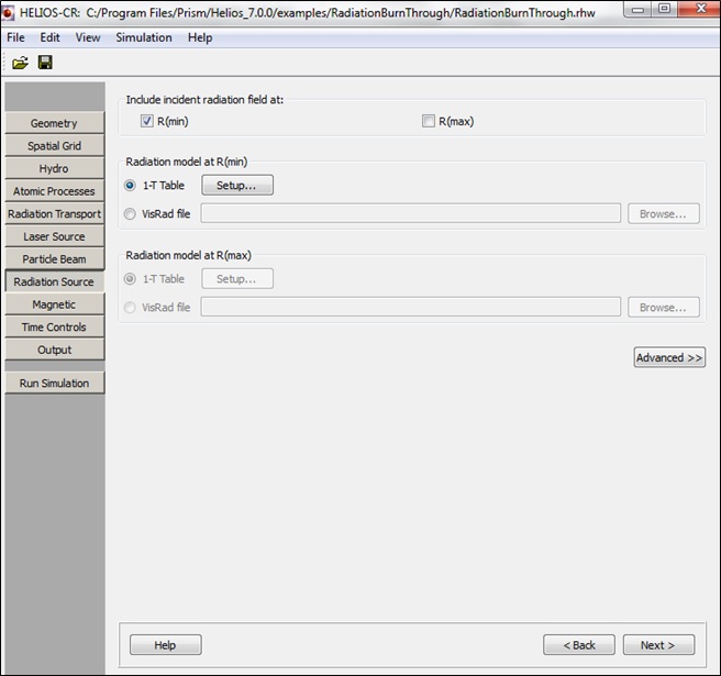
An external radiation source can be applied to the hydro grid boundaries during simulation. For planar geometries an external source can be applied at the inner boundary (R(min)) and/or the outer boundary (R(max)). For cylindrical and spherical geometries, an external source can only be applied at the outer boundary. The time-dependence of the flux is based on interpolated radiation temperatures from the 1 - T table. The photon energy-dependence is determined assuming a Planckian source with a temperature given by the radiation temperature.

1. Select Include incident radiation field at R(min) checkbox.
2. Select 1-T table radio button and click Setup.
3. Enter values 0, 1e-10, 2e-10 for time, and 0, 200, 200 for drive temperature.
4. Click OK.
5. Click Next.



7. If the Magnetic parameters are available, leave them unchanged and click Next.

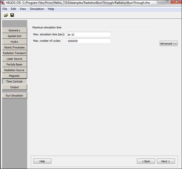
8. Setup Time Controls: enter 2e-10 in Max. simulation time field and click Next.

   

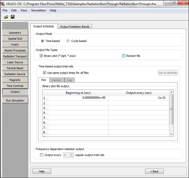
9. Setup Output: enter 1e-11 in the table (column Output every), save the file, and then press Run Simulation.

   

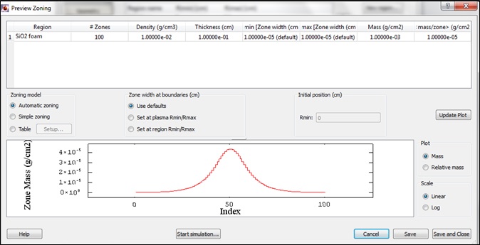
10. In Preview zoning dialog make sure that the zoning is good, and press Start simulation.

    

11. In the confirmation dialog select Run Directory, Run Name, and click OK.
    
    
12. Simulation starts.

Example Simulation Results: Electron temperature distribution in the foam at different times.