Example: Laser-Heated Foil

In this calculation, an 80 ns long laser beam (fluence: 50 J/cm2, wavelength: 1.054 mm) is used to accelerate an Al flyer.

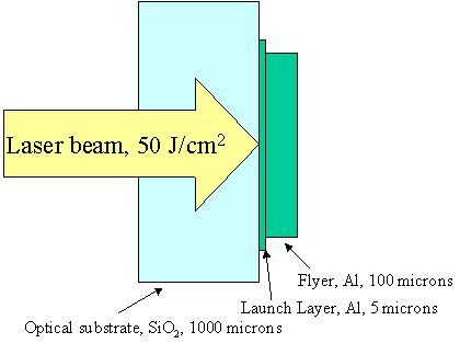
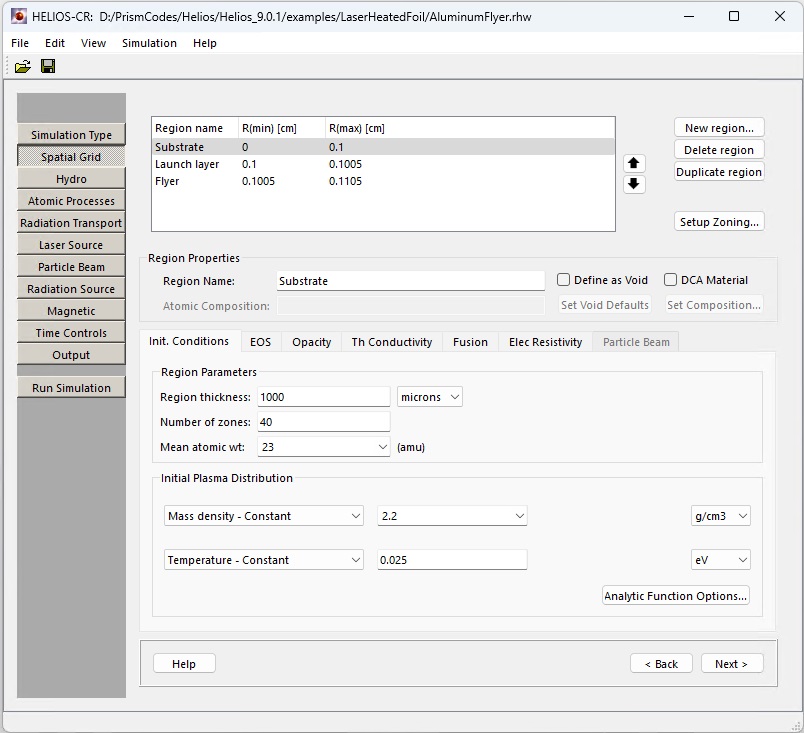
Setup:

1. Choose geometry: Planar, cylindrical and spherical geometries are supported. Calculations may be started with non-zero minimum node position, may be useful for modeling implosions. Select Planar and click Next.
   
   
2. Setup Spatial Grid. The regions in the regions box are ordered according to their position in the grid. To change the position of a region (relative to another existing region), select the region and apply either the up or down arrow on the right side of the regions box. The minimum and maximum radii for each of the regions are then automatically updated. The steps for this relatively complex dialog are:
   
   
1. Click New region.
   


2. Set region properties.
·       In Region name enter Substrate.
·       In the Init. Conditions tab, for Thickness: enter 1000, and select microns from the dropdown menu.
·       Mass density: select SiO₂ from the dropdown menu.
·       Number of zones: enter 40.
·       Mean atomic weight: select SiO₂ from the dropdown menu.
·       Temperature: leave at the default of 0.025 eV (room temperature).





3. Select EOS table. Supported EOS models are SESAME (fiels must be obtained from LANL), PROPACEOS and Ideal gas.
·       Click on EOS tab.
·       Make sure that Equation of state type PROPACEOS and Location Library are selected.
·       In EOS file dropdown menu select SiO2.prp.






4. Select Opacity table.
·       Click on Opacity tab.
·       Make sure that Opacity data type PROPACEOS and Location Library are selected.
·       In Opacity file dropdown menu select SiO2.prp.






5. Select conductivity model.
   

   Constant conductivity model: conductivity for that spatial region is set to the value entered by the user.

   Hybrid conductivity model: parameters are entered into the dialog box.

   Spitser: conductivites are used in all temperature-density space except that representation of a solid. Users define the temperature and density bounding the solid phase. Specifically, at densities above some minimum density, r(min), and at temperatures below some maximum temperature T(max) the conductivit is set to the solid conductivity value specified by the user.

   ·       Click on Conductivity tab.
   ·       Select Hybrid radio button and click Set parameters...
   ·       In the new dialog box fill in corresponding fields:
   ·       Solid conductivity: enter 1.
   ·       Max. temperature: enter 1.
   ·       Min. density: enter 1.
   ·       Click OK.
   
   
6. Select tab Init. Conditions and click New region again.
   
   
7. Set region properties.
·       In Region name enter Launch layer.
·       Thickness: enter 5, and select microns from the dropdown menu.
·       Mass density: select Al-solid  from the dropdown menu.
·       Number of zones: enter 20.
·       Mean atomic weight: select Al-solid  from the dropdown menu.
·       Temperature: leave at the default of 0.025 eV (room temperature).
·       Velocity: leave at the default of 0.


8. Select EOS table.
·       Click on EOS tab.
·       Make sure that Opacity data type PROPACEOS and that Equation of state type and Location Library are selected.
·       In EOS file dropdown menu select Al.prp.


9. Select Opacity table.
   
·       Click on Opacity tab.
·       Make sure that Opacity data type PROPACEOS and Location Library are selected.
·       In Opacity file dropdown menu select Al.prp.


10. Select conductivity model.
    ·       Click on Conductivity tab.
    ·       Select Hybrid radio button and click Set parameters...
    ·       In the new dialog box fill in corresponding fields:
    ·       Solid conductivity: enter 250.
    ·       Max. temperature: enter 1.
    ·       Min. density: enter 0.27.
    ·       Click OK.
    
    
11. Select tab Init. Conditions and click Duplicate region.
    
    
12. Set region properties.
·       In Region name enter Flyer.
·       Thickness: enter 100, and select microns from the dropdown menu.
·       Number of zones: enter 40.


13. After setting up each of the spatial regions, the zoning (or mass distribution of zones) must be set up. In most cases, this can be accomplished using the Automatic Zoning option. For a Lagrangian code, it is important to have a smooth distribution of zone masses. Generally, relative mass differences between two adjacent zones should be within a few tens of percent.
    
    Click Setup Zoning. The Preview Zoning window will open.
    
    
14. In the Preview Zoning:
    
·       Uncheck Use defaults checkbox.
·       Select Set at plasma Rmin/Rmax radio button in the Zone width at boundaries (cm), and update the Rmin and Rmax values as shown below.
·       Click the Update Plot button and make sure that the mass distribution is smooth.
·       Click Save and Close.






15. Click Next.
    
    

3. Choose hydro calculation mode (one-temperature): select T(ion)=T(electron) and click Next.
   

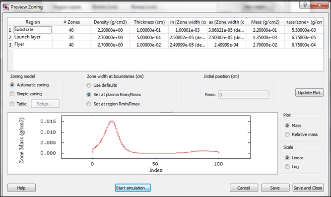
   T(ion) = T(electron) button: energy equations are solved such that the ion and electron temperatures are the same. Otherwise, the ion and electron temperatures are obtained using a two-temperature solution of the energy conservation equations. 1-T calculations generally run faster, and users may want to use this option when they do not expect electrons and ions to be strongly decoupled. It may also be advantageous to use the 1-T model for low energy density systems.

   Quiet start refers to holding the hydro grid in place until a threshold temperature is attained. This, for example, can prevent a cold fluid (i.e., gas or plasma) from slowly expanding into a vacuum due to its own pressure. If used, typically a quiet start temperature of a fraction of an eV is used.

   Boundary conditions: usually the boundaries of the plasma are allowed to expand freely. If required, the boundaries can be held stationary by unchecking the Rmin and/or Rmax boxes.

   Artificial viscosity: there is an option to use a multiplier on the artificial viscosity values.

   Please note that all options in Atomic Processes will be grayed out because we did not select a DCA model in the Spacial Grid step.
   
   
4. In Radiation Transport setup leave the defaults unchanged and click Next.
   
   
5. Setup Laser Source.
   
   
1. Turn on and configure laser properties.
·       Check Include laser 1 checkbox.
·       Select Interior region radio button. Note that a laser source can originate from the inner or outer boundary of the hydro grid -- i.e., R(min) or R(max) -- or at the boundary between any two spatial regions.
·       Choose Launch layer at R(min) from the dropdown menus (Note that in the calculation, the optical substrate may not be transparent to the laser light, and the laser source must be therefore applied to the inner launch layer surface).
·       In Beam Parameters enter laser wavelength: 1.054.


2. Configure laser beam power.
·       Click Setup.
·       In the new window select File, then Import Data.
·       Navigate to file Laser50.DAT (this file is supplied with the distribution) and click open.
·       Click OK in the confirmation dialog.
·       Click OK in the Laser Powers setup dialog.


3. Click Next.
   

   

   
   

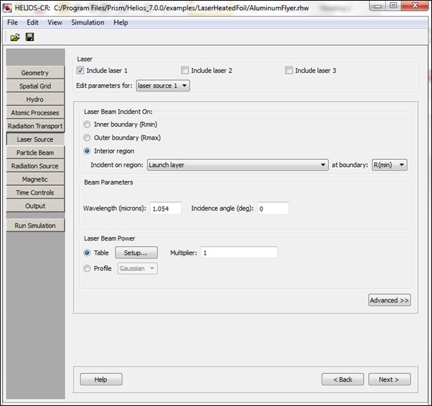
6. Leave Radiation Source parameters unchanged and click Next.

7. If the Magnetic parameters are available, leave them unchanged and click Next.
   
   
8. Setup Time Controls: enter 2e-7 in Max. simulation time field and click Next.
   
   
9. Setup Output: select Time-based Output Mode, enter 5e-9 for the Output every (sec): in the table, Save the file, and then press Run Simulation.
   
   
10. In Preview zoning dialog, verify the zoning is satisfactory; then press Start simulation.
    
    
11. In the confirmation dialog select Run Directory, Run Name, and click OK.
    
    
12. The simulation now starts.

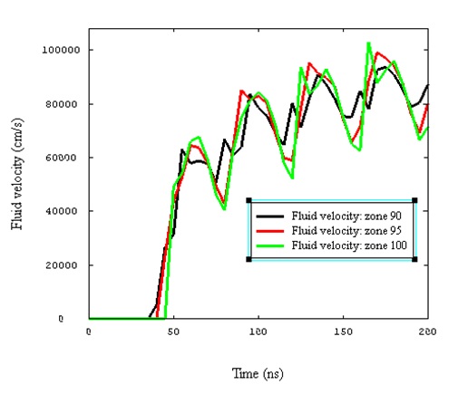
Example Simulation Results: Time evolution of velocity in individual zones in the vicinity of the flyer plate boundary.