Example: Radiation-Heated Al Foil

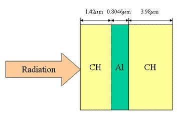
In this calculation, radiation heats a plastic-tamped Al foil.

Setup:

1. Choose geometry: select Planar and click Next.

2. Setup Spatial Grid. The steps for this relatively complex dialog are:

1. Click New region.

2. Set region properties.
   • In Region name enter Al.
   • In Init. Conditions tab, for Thickness: enter 0.8046, and select microns from dropdown menu.
   • Mass density-Constant: select Al-solid from the dropdown menu.
   • Number of zones: enter 20.
   • Mean atomic weight: select Al-solid from the dropdown menu.
   • Select Mass Density - constant and select Al-solid from the dropdown menu.
   • Temperature: enter 0.3.

   

3. Select EOS table.
   • Click on EOS tab.
   • Make sure that Equation of state type PROPACEOS and Location Library are selected.
   • In EOS file dropdown menu select Al.prp.
   
   
4. Select Opacity table
   • Click on Opacity tab.
   • Make sure that Opacity data type PROPACEOS and Location Library are selected.
   • In Opacity file dropdown menu select Al.prp.

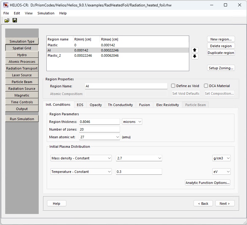
5. Select tab Init. Conditions and click New region again.

6. Set region properties.
   • In Region name enter Plastic.
   • Thickness: enter 1.42, and select microns from the dropdown menu.
   • Mass density: select CH-polystyrene  from the dropdown menu.
   • Number of zones: enter 50.
   • Mean atomic weight: select CH-polystyrene from the dropdown menu.
   • Temperature: enter 0.3.
   • Velocity: leave at the default of 0.
   
   
7. Select EOS table.
   • Click on EOS tab.
   • Make sure that Equation of state type PROPACEOS and Location Library are selected.
   • In EOS file dropdown menu select CH.prp.

   

   
   
8. Select Opacity table.
   • Click on Opacity tab.
   • Make sure that Opacity data type PROPACEOS and Location Library are selected.
   • In Opacity file dropdown menu select CH.prp.

9. Select tab Init. Conditions and click Duplicate region.

10. Set region properties.
    • Thickness: enter 3.98.
    • Number of zones: enter 30.

11. Use up and down arrows to arrange the materials in the following order: Plastic, Al, Plastic_2.

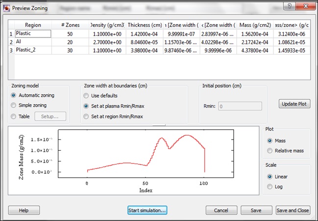
12. Select tab Init. Conditions and click setup zoning.

13. In Zoning dialog:
    • Uncheck Use defaults checkbox.
    • Select Set at plasma Rmin/Rmax radio button.
    • For Plastic, enter 1e-6 for Rmin, and 2.83997e-6 for Rmax.
    • For Al, enter 1.15703e-6 for Rmin, and 4.02298e-6 for Rmax.
    • For Plastic_2, enter 9.87460e-6 for Rmin, and 1e-5 for Rmax.
    • Click Update Plot and make sure that the mass distribution is smooth.
    • Click Save and Close.

    

    
    
14. Click Next.

3. Choose hydro calculation mode (one-temperature):
1. Select T(ion) = T(electron).
2. Click Advanced button and enter 0.4 for the quiet start temperature.
3. Click Next.


4. In Radiation Transport setup:

The radiation transport is performed using one of the following: a multi-group, flux-limited Diffusion model (most commonly used in rad-hydro codes), or a multi-group, Multiangle long characteristics model (more accurate, but potentially slower), or None – radiation transport is ignored. The radiation heating and cooling will still be computed. At present, the multi-angle model can be utilized only in planar geometry.

The binning, or distribution, of frequency (i.e., photon energy) groups is set up using one of the following approaches. Typical: using the specified number of frequency groups, a grid is set up with approximately 85% of the groups having photon energies between 0.1 eV and 3 KeV, while the remaining 15% lie between 3 KeV and 1 MeV. Tabulated Group Boundaries: the boundaries of the frequency groups are entered into a table or the table values can be imported from a file. Specify Frequency Groups in Sections: the spectrum is divided into "sections" (or spectral ranges), the number of which is given by the number of filled table rows. For each section, the number of groups and the upper bound of each section of groups is specified. This allows the user to specify high frequency resolution in one spectral range, and a coarser frequency resolution in another range.

1. Make sure that Multiangle radiation transport model is selected.
2. Enter 2 for the Number of angles .
3. Enter 100 for the number of frequency groups.
4. Click Next.

5. Leave Laser Source parameters unchanged and click Next.

6. Setup Radiation Source parameters.
1. Select Include incident radiation field at R(min) checkbox.
2. Select 1-T table radio button and click Setup.
3. In the new window select File, then Import Data.
4. Navigate to file Radiation_temperatures.dat (this file is supplied with the distribution) and click Open.
5. Click OK.
6. Click Next.

7. If the Magnetic parameters are available, leave them unchanged and click Next.

8. Setup Time Controls: enter 1.1e-7 in Max. simulation time field and click Next.

9. Setup Output: enter 0 and 8e-8 in the column Beginning at and 2e-9, 5e-10 in the column Output every, save the file, and then press Run Simulation.

10. In Preview zoning dialog make sure that zoning is good, and press Start simulation.

11. In the confirmation dialog select Run directory, Run name, and click OK.

12. Simulation starts.

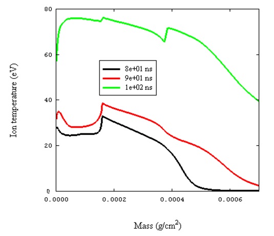
Example Simulation Results: Plasma temperature distribution at three different time steps.