Example: Radiation-Driven Capsule Implosion

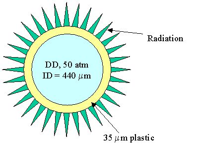
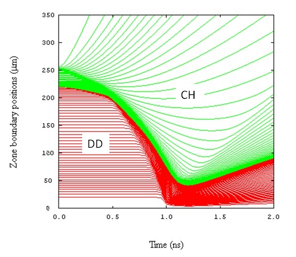
In this calculation, a plastic micro balloon (wall thickness - 35 micron, internal diameter - 220 micron) is filled with 50 atm DD. The capsule is driven by 200 eV radiation for 1 nanosecond. This system is representative of indirectly driven capsule implosion experiments at OMEGA.

Setup:

1. Choose geometry: select Spherical and click Next.

2. Setup Spatial Grid. The steps for this relatively complex dialog are:

1. Click New region.

2. Set region properties.
   • In Region name enter DD.
   • In the Init. Conditions tab, enter Thickness: enter 220, and select microns from the dropdown menu.
   • Mass Density - constant: enter 0.0085 (Mass density of DD at 50 atm).
   • Number of zones: enter 50.
   • Mean atomic weight: enter 2.
   • Temperature: leave at default value of 0.025 eV (room temperature).

   



3. Select EOS table.
   • Click on EOS tab.
   • Make sure that Equation of state type PROPACEOS and Location Library are selected.
   • In EOS file dropdown menu select DT.prp.

   



4. Select Opacity table
   • Click on Opacity tab.
   • Make sure that Opacity data type PROPACEOS and Location Library are selected.
   • In Opacity file dropdown menu select DT.prp

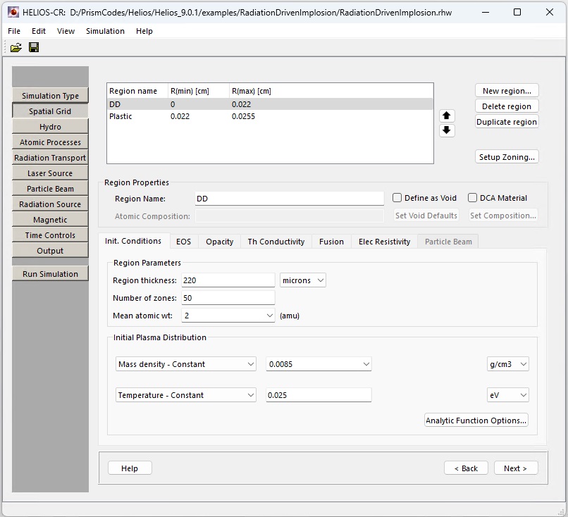
5. Select tab Init. Conditions and click New region again.

6. Set region properties.
   • In Region name enter Plastic.
   • Thickness: enter 35, and select microns from the dropdown menu.
   • Mass density: select CH-polystyrene  from the dropdown menu.
   • Number of zones: enter 50.
   • Mean atomic weight: select CH-polystyrene from the dropdown menu.
   • Temperature: leave at default value of 0.025 eV (room temperature).
   • Velocity: leave at default value of 0.
     


7. Select EOS table.
   • Click on EOS tab.
   • Make sure that Equation of state type PROPACEOS and Location Library are selected.
   • In EOS file dropdown menu select CH.prp.
   
   
8. Select Opacity table.
   • Click on Opacity tab.
   • Make sure that Opacity data type PROPACEOS and Location Library are selected.
   • In Opacity file dropdown menu select CH.prp.

9. Select tab Init. Conditions and click setup zoning.

10. In Zoning dialog:
    • Uncheck Use defaults checkbox.
    • Select Set at plasma Rmin/Rmax checkbox.
    • For DD material, enter 0.002 for Rmin, and 1.47652e-4 for Rmax.
    • For Plastic enter 1.1308e-6 for Rmin, and 6.09766e-5 for Rmax.
    • Click Update zoning and make sure that the mass distribution is smooth.
    • Click Save and Close.
    
    
11. Click Next.

3. Choose hydro calculation mode (two-temperature):
1. Select T(ion) < >T(electron).
2. Click Advanced button and enter 0.1 for quiet start temperature.
3. Click Next.


4. In Radiation Transport setup:

The radiation transport is performed using one of the following: a multi-group, flux-limited Diffusion model (most commonly used in rad-hydro codes), or a multi-group, Multiangle long characteristics model (more accurate, but potentially slower), or None – radiation transport is ignored. The radiation heating and cooling will still be computed. At present, the multi-angle model can be utilized only in planar geometry.

The binning, or distribution, of frequency (i.e., photon energy) groups is set up using one of the following approaches. Typical: using the specified number of frequency groups, a grid is set up with approximately 85% of the groups having photon energies between 0.1 eV and 3 KeV, while the remaining 15% lie between 3 KeV and 1 MeV. Tabulated Group Boundaries: the boundaries of the frequency groups are entered into a table or the table values can be imported from a file. Specify Frequency Groups in Sections: the spectrum is divided into "sections" (or spectral ranges), the number of which is given by the number of filled table rows. For each section, the number of groups and the upper bound of each section of groups is specified. This allows the user to specify high frequency resolution in one spectral range, and a coarser frequency resolution in another range.

1. Make sure that Diffusion radiation transport model is selected.
2. Enter 100 for the number of frequency groups.
3. Click Next.



5. Leave Laser Source parameters unchanged and click Next.

6. Setup Radiation Source parameters.
1. Select Include incident radiation field at R(max) checkbox.
2. Select 1-T table radio button and click Setup.
3. In the table enter 0.0 and 1.0e-9 for time, and 200 for drive temperature at both times.
4. Click OK.
5. Click Next.

7. If the Magnetic parameters are available, leave them unchanged and click Next.

8. Setup Time Controls: enter 3e-9 in Max. simulation time field and click Next.

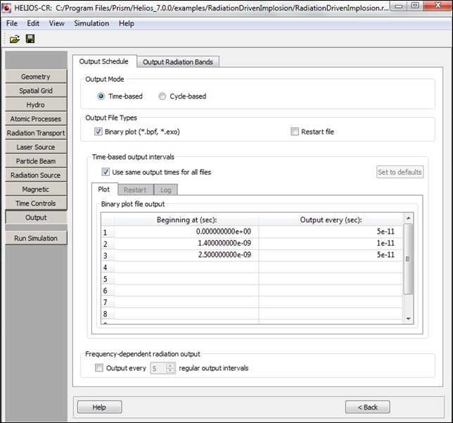
9. Setup Output: enter table values as shown below, save the file, and then press Run Simulation.

   

10. In Preview zoning dialog make sure that the zoning is good, and press Start simulation.

11. In the confirmation dialog select Run directory, Run name, and click OK.

12. Simulation starts.

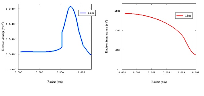
Simulation Results: Plasma core temperature and density distributions around the time of implosion stagnation (1.1 ns).